Multi-Layer Perceptron Networks in Theano and TensorFlow: An Implementation and Benchmark

Sat, 15 Apr 2017

Ai, Ann, Benchmark, Computer Science, Machine Learning, Mlp, Python, Tensorflow, Theano

A past blog post explored using multi-layer-perceptrons (MLP) to predict stock prices using Tensorflow and Python. This post introduces another common library used for artificial neural networks (ANN) and other numerical purposes: Theano. An MLP Python class is created implemented using Theano, and then the performance of the class is compared with the TFANN class in a benchmark.

Installing Theano on Windows

An easy way to get Theano working quickly is to first install Anaconda. Anaconda is packaged with Python, NumPy, and several other of the installation requirements bundled together in a convenient installer (see Figure 1). This guide recommends using Anaconda3-4.2.0 for 64-bit Windows for simultaneous compatibility with TensorFlow.

Figure 1: Anaconda Python Installer

An additional dependency that is required is a GCC toolchain. If the computer has an existing version of GCC or G++ installed, environment variables may need to be set to ensure Theano uses the appropriate tool chain. In Windows, environment variables can be viewed by typing set at the command prompt. System environment variables can be modified under System -> Change Settings -> Advanced -> Environment Variables (on Server 2012 R2). User environment variables are set under User Accounts -> Change my environment variables. If there are no conflicting GCC toolchains (mingw, mingw64, etc), the m2w64-toolchain can be installed by typing: conda install m2w64-toolchain at an Anaconda Command Prompt. This will make G++ in the Anaconda Prompt (a special command prompt including extra environment variables that is bundled with Anaconda).

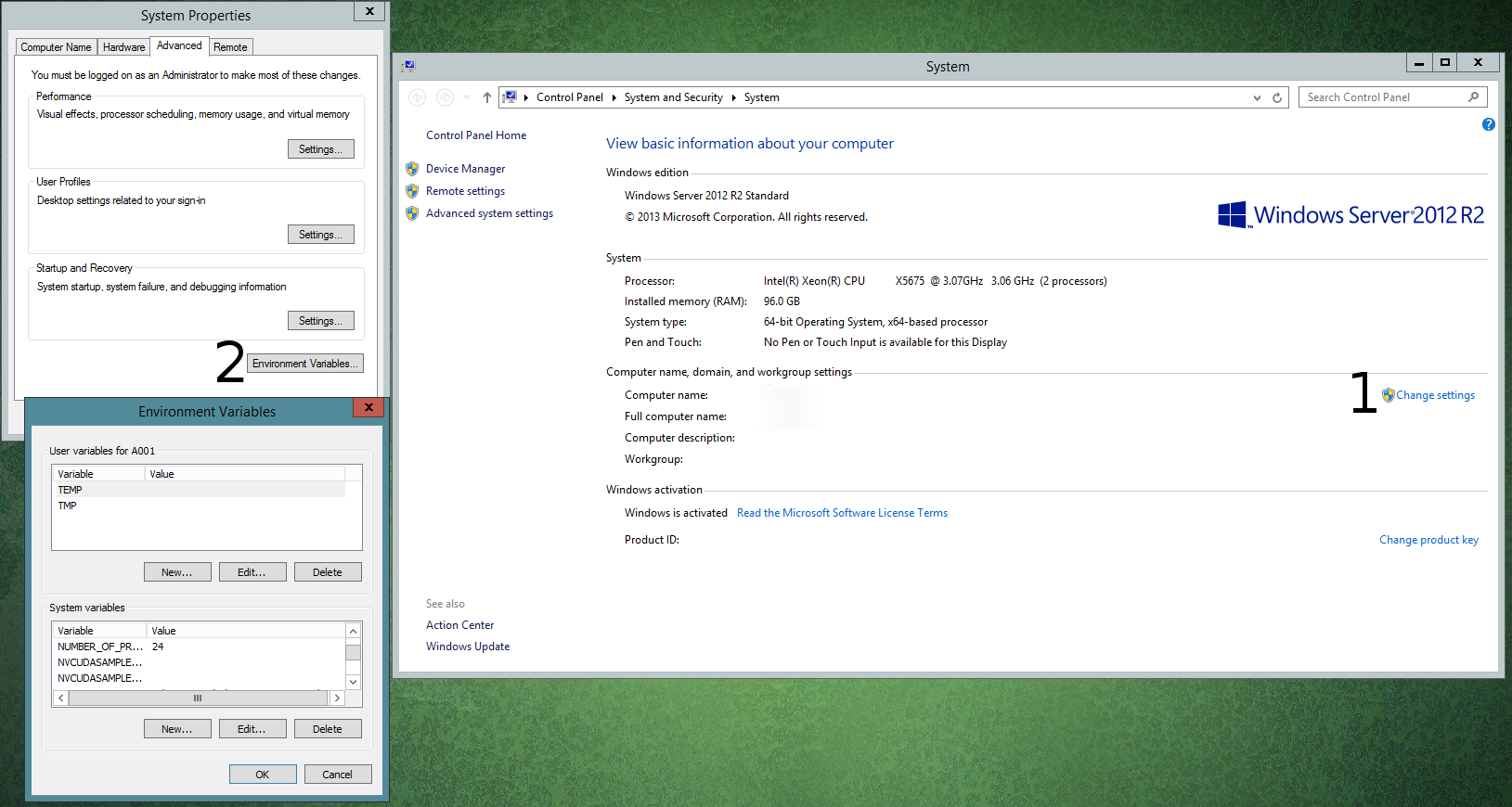
Figure 2: Setting System Environment Variables in Windows

If the computer has an NVidia GPU with CUDA Compute Capability of 1.2 or greater, Theano can be configured to run on the GPU. NVidia's website has a page that lists the Compute Capability for each of their supported cards. CUDA can be downloaded here. Note: CUDA recommends installing Visual Studio for full support. Visual Studio 2010 was used for this guide.

With the above dependencies installed, Theano can be installed by typing: conda install theano pygpu at an Anaconda Command Prompt. Note: At the time of writing this post, there is a memory leak issue in Theano 0.9.0 causing memory consumption to grow without bound. Version 0.8.2 does not have this issue and can be installed using conda install theano=0.8.2.

An MLP Class Using Theano

Similar to TensorFlow, most Theano functions create graph operations that are not immediately performed. This computation graph is later evaluated to perform the actual desired operations.

In this class, the MLP network is constructed using the typical matrix multiplication representation. The output of a layer is the matrix product of the input matrix with the weight matrix. A bias term is added to the output and then an activation function is applied element-wise on the result. For more details about the math behind MLP networks, see a past blog post. Code to setup the MLP class is as follows:

---

#Create an MLP: A sequence of fully-connected layers with an activation
#function AF applied at all layers except the last.
#X:		The input tensor
#W:		A list of weight tensors for layers of the MLP
#B:		A list of bias tensors for the layers of the MLP
#AF: 	The activation function to be used at hidden layers
#Ret:	The network output 
def CreateMLP(X, W, B, AF):
	n = len(W)
	for i in range(n - 1):
		X = AF(X.dot(W[i]) + B[i])
	return X.dot(W[n - 1]) + B[n - 1]

#Creates weight and bias matrices for an MLP network
#given a list of the layer sizes.
#L:		A list of the layer sizes
#Ret:	The lists of weight and bias matrices (W, B)
def CreateMLPWeights(L):
	W, B = [], []
	n = len(L)
	for i in range(n - 1):
		#Use Xavier initialization for weights
		xv = np.sqrt(6. / (L[i] + L[i + 1]))
		W.append(theano.shared(np.random.uniform(-xv, xv, [L[i], L[i + 1]])))
		#Initialize bias to 0
		B.append(theano.shared(np.zeros([L[i + 1]])))
	return (W, B)  

#Given a string of the activation function name, return the
#corresponding Theano function.
#Ret:	The Theano activation function handle
def GetActivationFunction(name):
	if name == 'tanh':
		return T.tanh
	elif name  == 'sig':
		return T.nnet.sigmoid
	elif name == 'fsig':
		return T.nnet.ultra_fast_sigmoid
	elif name == 'relu':
		return T.nnet.relu
	elif name == 'softmax':
		return T.nnet.softmax

class TheanoMLPR:

	def __init__(self, layers, actfn = 'tanh', batchSize = None, learnRate = 1e-3, maxIter = 1000, tol = 5e-2, verbose = True):
		self.AF = GetActivationFunction(actfn)
		#Batch size
		self.bs = batchSize
		self.L = layers
		self.lr = learnRate
		#Error tolerance for early stopping criteron
		self.tol = tol
		#Toggles verbose output
		self.verbose = verbose
		#Maximum number of iterations to run
		self.nIter = maxIter
		#List of weight matrices
		self.W = []
		#List of bias matrices
		self.B = []
		#Input matrix
		self.X = T.matrix()
		#Output matrix
		self.Y = T.matrix()
		#Weight and bias matrices
		self.W, self.B = CreateMLPWeights(layers)
		#The result of a forward pass of the network
		self.YH = CreateMLP(self.X, self.W, self.B, self.AF)
		#Use L2 loss for network
		self.loss = ((self.YH - self.Y) ** 2).mean()
		#Function for performing a forward pass
		self.ffp = theano.function([self.X], self.YH)
		#For computing the loss
		self.fcl = theano.function([self.X, self.Y], self.loss)
		#Gradients for weight matrices
		self.DW = [T.grad(self.loss, Wi) for Wi in self.W]
		#Gradients for bias
		self.DB = [T.grad(self.loss, Bi) for Bi in self.B]
		#Weight update terms
		WU = [(self.W[i], self.W[i] - self.lr * self.DW[i]) for i in range(len(self.DW))]
		BU = [(self.B[i], self.B[i] - self.lr * self.DB[i]) for i in range(len(self.DB))]
		#Gradient step
		self.fgs = theano.function([self.X, self.Y], updates = tuple(WU + BU))

---

As can be seen above, the network graph is created in the constructor for the TheanoMLPR class. Note that self.X and self.Y are placeholders for the input matrices, similar to TensorFlow. theano.function is used to create a function in the computation graph which is used to provide input and get output from the graph itself. For instance, self.ffp = theano.function([self.X], self.YH) creates a function that takes as input self.X and performs the necessary operations to get self.YH using self.X as input. self.YH is defined as the feedforward step (see CreateMLP), so self.ffp therefore performs the feedforward process in the MLP.

Fitting the network is done similar to the corresponding MLPR TensorFlow class. On each training iteration the gradients are computed for the network and then applied to the weight and bias matrices using self.fgs. Prediction and scoring are simple applications of the function defined in the constructor. The remaining code for the class is as follows:

---

#Initializes the weight and bias matrices of the network
def Initialize(self):
	n = len(self.L)
	for i in range(n - 1):
		#Use Xavier initialization for weights
		xv = np.sqrt(6. / (self.L[i] + self.L[i + 1]))
		self.W[i].set_value(np.random.uniform(-xv, xv, [self.L[i], self.L[i + 1]]))
		#Initialize bias to 0
		self.B[i].set_value(np.zeros([self.L[i + 1]]))		
		
#Fit the MLP to the data
#A: 	numpy matrix where each row is a sample
#Y: 	numpy matrix of target values
def fit(self, A, Y):
	self.Initialize()
	m = len(A)
	for i in range(self.nIter):
		if self.bs is None: #Use all samples
			self.fgs(A, Y)			#Perform the gradient step
		else: 	#Train m samples using random batches of size self.bs
			for _ in range(0, m, self.bs):
				#Choose a random batch of samples
				bi = np.random.randint(m, size = self.bs)
				self.fgs(A[bi], Y[bi])	#Perform the gradient step on the batch
		if i % 10 == 9:
			loss = self.score(A, Y)
			if self.verbose:
				print('Iter {:7d}: {:8f}'.format(1 + i, loss))
			if loss < self.tol:
				break

#Predict the output given the input (only run after calling fit)
#A: 	The input values for which to predict outputs
#Ret: 	The predicted output values (one row per input sample)
def predict(self, A):
	return self.ffp(A)

#Predicts the ouputs for input A and then computes the loss term
#between the predicted and actual outputs
#A: 	The input values for which to predict outputs
#Y: 	The actual target values
#Ret: 	The network loss term
def score(self, A, Y):
	return np.float64(self.fcl(A, Y))

---

The complete code for the class is available here on GitHub.

Tensorflow vs Theano Benchmark

Next, a benchmark is constructed to compare the performance of the TheanoMLPR class with that of the MLPR class from TFANN developed earlier. A data set comprised of random data is generated. Target values are taken to be the sum of the corresponding sample vectors squared. The sample matrix is then perturbed by values in [0, 1] and scaled again to the range [0, 1]. The sample and target matrices are written to a file so that both benchmarks can use identical data sets.

---

#Generate data with nf features and ns samples. If new data
#is generated, write it to file so it can be reused across all benchmarks
def GenerateData(nf = 256, ns = 16384):
	try:	#Try to read data from file
		A = np.loadtxt('bdatA.csv', delimiter = ',')
		Y = np.loadtxt('bdatY.csv', delimiter = ',').reshape(-1, 1)
	except OSError:		#New data needs to be generated
		x = np.linspace(-1, 1, num = ns).reshape(-1, 1)
		A = np.concatenate([x] * nf, axis = 1)
		Y = ((np.sum(A, axis = 1) / nf) ** 2).reshape(-1, 1)
		A = (A + np.random.rand(ns, nf)) / (2.0)
		np.savetxt('bdatA.csv', A, delimiter = ',')
		np.savetxt('bdatY.csv', Y, delimiter = ',')
	return (A, Y)

---

The benchmark compares the time taken for each model in training and testing. The amount of time to train and test each model is measured as the number of samples in the data set increases. The original data set is divided into n pieces and the training and testing times using the first i chunks are recorded.

---

#R:		Regressor network to use
#A:		The sample data matrix
#Y:		Target data matrix
#nt:	Number of times to divide the sample matrix
#fn:	File name to write results
def MakeBenchDataFeature(R, A, Y, nt, fn):
	#Divide samples into nt peices on for each i run benchmark with chunks 0, 1, ..., i
	step = A.shape[1] // nt
	TT = np.zeros((nt, 3))
	for i in range(1, nt):
		#Number of features
		TT[i, 0] = len(range(0, (i * step)))
		print('{:8d} feature benchmark.'.format(int(TT[i, 0])))
		#Training and testing times respectively
		TT[i, 1], TT[i, 2] = RunBenchmark(R, A[:, 0:(i * step)], Y[:, 0:(i * step)])
	#Save benchmark data to csv file
	np.savetxt(fn, TT, delimiter = ',', header = 'Samples,Train,Test')
	
#Plots benchmark data on a given matplotlib axes object
#X:		X-axis data
#Y:		Y-axis data
#ax:	The axes object
#name:	Name of plot for title
#lab:	Label of the data for the legend
def PlotBenchmark(X, Y, ax, xlab, name, lab):
	ax.set_xlabel(xlab)
	ax.set_ylabel('Avg. Time (s)')
	ax.set_title(name + ' Benchmark')
	ax.plot(X, Y, linewidth = 1.618, label = lab)
	ax.legend(loc = 'upper left')
	
#Runs a benchmark on a MLPR model 
#R:		Regressor network to use
#A:		The sample data matrix
#Y:		Target data matrix
def RunBenchmark(R, A, Y):
	#Record training times
	t0 = time.time()
	R.fit(A, Y)
	t1 = time.time()
	trnt = t1 - t0
	#Record testing time
	t0 = time.time()
	YH = R.predict(A)
	t1 = time.time()
	tstt = t1 - t0
	return (trnt, tstt)

---

To allow for a more fair comparison, the main program performs a single benchmark on each run. This is accomplished by passing a command-line argument to the program to indicate which benchmark to run: tensorflow, theanogpu, or theano. The command-line argument plot will display the generated benchmark data and plot it using MatPlotLib.

---

def Main():
	if len(sys.argv) <= 1:
		return
	A, Y = GenerateData(ns = 2048)
	#Create layer sizes; make 6 layers of nf neurons followed by a single output neuron
	L = [A.shape[1]] * 6 + [1]
	print('Layer Sizes: ' + str(L))
	if sys.argv[1] == 'theano':
		print('Running theano benchmark.')
		from TheanoANN import TheanoMLPR
		#Create the Theano MLP
		tmlp = TheanoMLPR(L, batchSize = 128, learnRate = 1e-5, maxIter = 100, tol = 1e-3, verbose = True)
		MakeBenchDataSample(tmlp, A, Y, 16, 'TheanoSampDat.csv')
		print('Done. Data written to TheanoSampDat.csv.')
	if sys.argv[1] == 'theanogpu':
		print('Running theano GPU benchmark.')
		#Set optional flags for the GPU
		#Environment flags need to be set before importing theano
		os.environ["THEANO_FLAGS"] = "device=gpu"
		from TheanoANN import TheanoMLPR
		#Create the Theano MLP
		tmlp = TheanoMLPR(L, batchSize = 128, learnRate = 1e-5, maxIter = 100, tol = 1e-3, verbose = True)
		MakeBenchDataSample(tmlp, A, Y, 16, 'TheanoGPUSampDat.csv')
		print('Done. Data written to TheanoGPUSampDat.csv.')
	if sys.argv[1] == 'tensorflow':
		print('Running tensorflow benchmark.')
		from TFANN import MLPR
		#Create the Tensorflow model
		mlpr = MLPR(L, batchSize = 128, learnRate = 1e-5, maxIter = 100, tol = 1e-3, verbose = True)
		MakeBenchDataSample(mlpr, A, Y, 16, 'TfSampDat.csv')
		print('Done. Data written to TfSampDat.csv.')
	if sys.argv[1] == 'plot':
		print('Displaying results.')
		try:
			T1 = np.loadtxt('TheanoSampDat.csv', delimiter = ',', skiprows = 1)
		except OSError:
			T1 = None
		try:
			T2 = np.loadtxt('TfSampDat.csv', delimiter = ',', skiprows = 1)
		except OSError:
			T2 = None
		try:
			T3 = np.loadtxt('TheanoGPUSampDat.csv', delimiter = ',', skiprows = 1)
		except OSError:
			T3 = None
		fig, ax = mpl.subplots(1, 2)
		if T1 is not None:
			PlotBenchmark(T1[:, 0], T1[:, 1], ax[0], '# Samples', 'Train', 'Theano')
			PlotBenchmark(T1[:, 0], T1[:, 2], ax[1], '# Samples', 'Test', 'Theano')
		if T2 is not None:
			PlotBenchmark(T2[:, 0], T2[:, 1], ax[0], '# Samples', 'Train', 'Tensorflow')
			PlotBenchmark(T2[:, 0], T2[:, 2], ax[1], '# Samples', 'Test', 'Tensorflow')	
		if T3 is not None:
			PlotBenchmark(T3[:, 0], T3[:, 1], ax[0], '# Samples', 'Train', 'Theano GPU')
			PlotBenchmark(T3[:, 0], T3[:, 2], ax[1], '# Samples', 'Test', 'Theano GPU')	
		mpl.show()

---

The completed code for the benchmark is available here on GitHub.

Results

The above code was run on a Z800 workstation running Windows Server 2012 R2. The system has the following configuration:

• 2x Intel Xeon X5675 Costa Rica @ 3.06Ghz
• 96GB PC3-10600R 1333MHz RAM
• 4x 300GB 15000RPM SAS Drives in RAID 0
• 2x NVidia Quadro 5000 2.5GB

The system is pictured below in Figure 3.

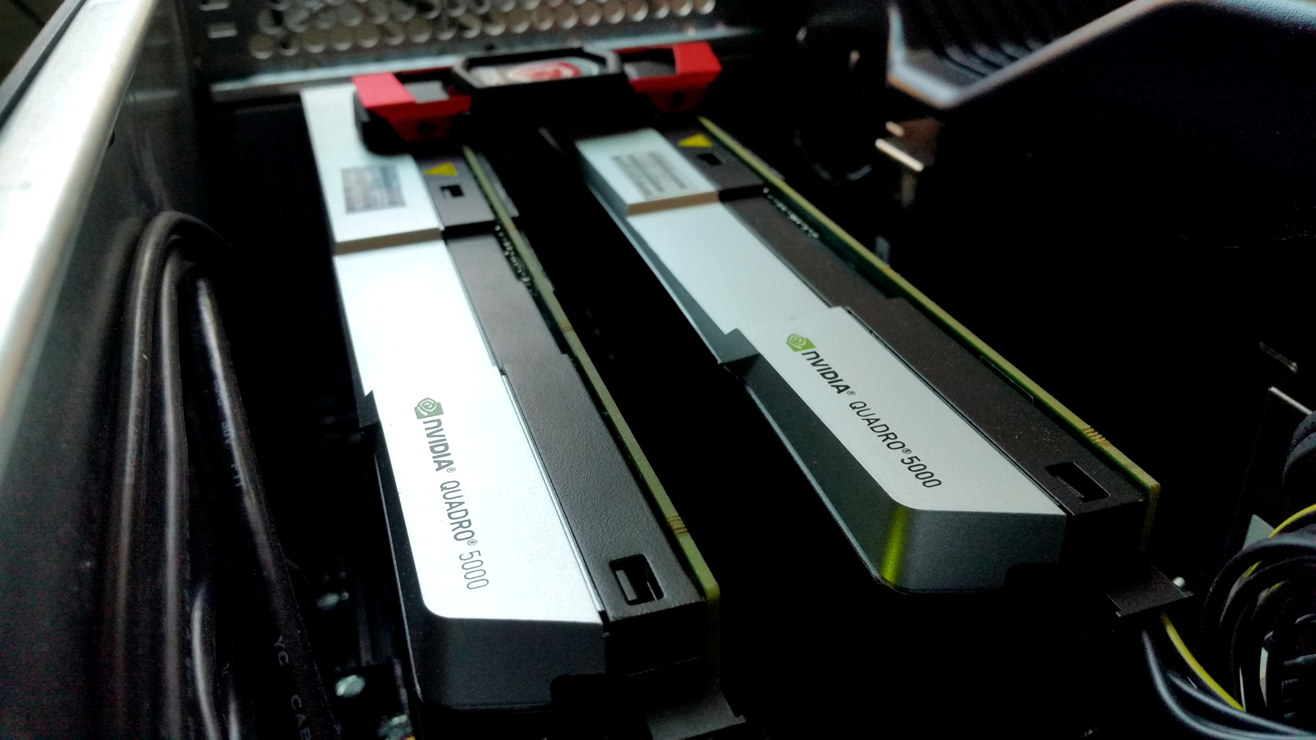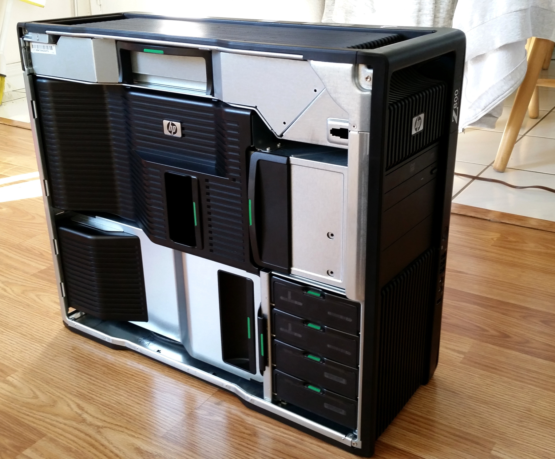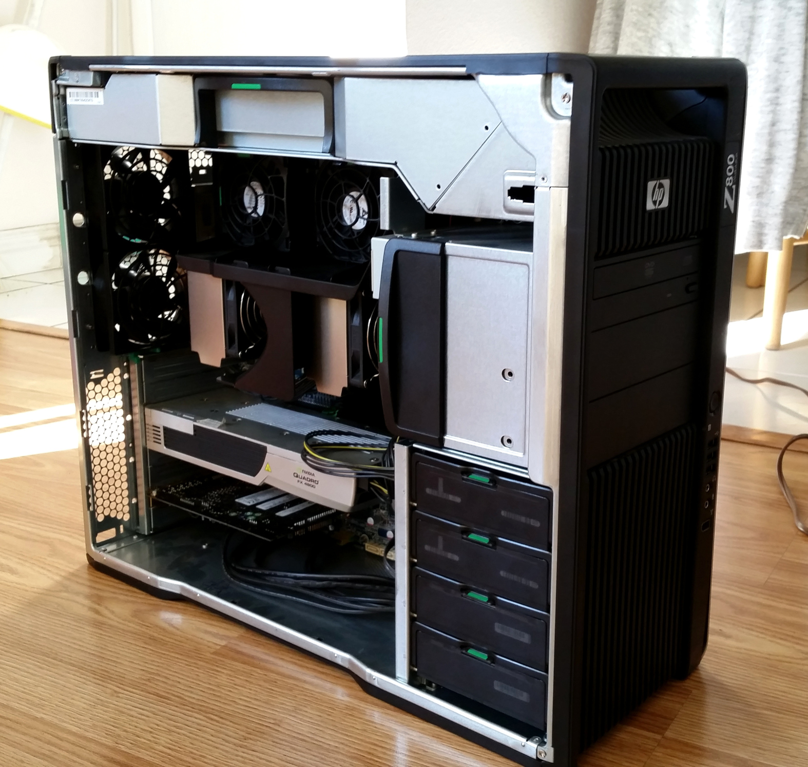Figure 3: The Benchmark Rig

The following commands can be used to generate the results and plots:

---

python Main.py theano
python Main.py theanogpu
python Main.py tensorflow
python Main.py plot

---

Note: For GPU based Theano, both the cl compiler and g++ must be in the PATH environment variable for the GPU to be used. This can be accomplished by running the vcvarsall.bat script that comes with Visual Studio inside an Anaconda prompt. The path to vcvarsall.bat may look similar to: C:\Program Files (x86)\Microsoft Visual Studio 10.0\VC\vcvarsall.bat. The plot generated by the program is shown below in Figure 4.

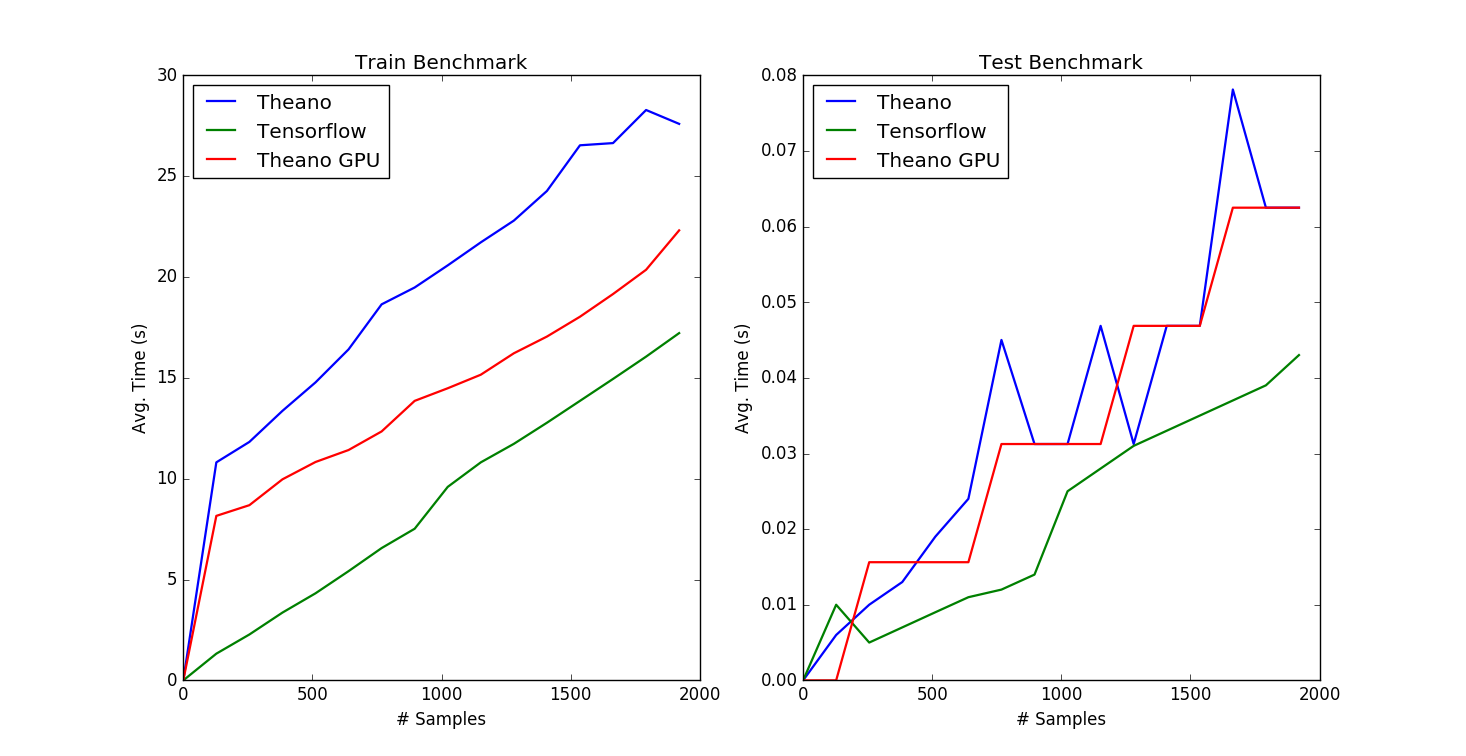
Figure 4: TensorFlow vs. Theano Benchmark Results

The above benchmark is constructed in an attempt to give a fair comparison between the two libraries, but it is by no means exhaustive. ANNs have numerous hyper-parameters and more benchmarks can be created to gain a better understanding of the performance trade-offs between TensorFlow and Theano. Due the CUDA Compute Capability of the Quadro 5000 being 2.0, the author is unable to benchmark GPU enabled TensorFlow.

The author is more than happy to include your benchmark results in this post if you share them below in a comment.