Multi-Layer Perceptrons and Back-Propagation; a Derivation and Implementation in Python
Sun, 27 Mar 2016
Computer Science, Machine Learning, Mathematics, Neural Networks, Numpy
Artificial neural networks have regained popularity in machine learning circles with recent advances in deep learning. Deep learning techniques trace their origins back to the concept of back-propagation in multi-layer perceptron (MLP) networks, the topic of this post. The complete code from this post is available on GitHub.Multi-Layer Perceptron Networks for Regression
A MLP network consists of layers of artificial neurons connected by weighted edges. Neurons are denoted \(n_{ij}\) for the \(j\)-th neuron in the \(i\)-th layer of the MLP from left to right top to bottom. Inputs are fed into the leftmost layer and propagate through the network along weighted edges until reaching the final, or output, layer. An example of a MLP network can be seen below in Figure 1.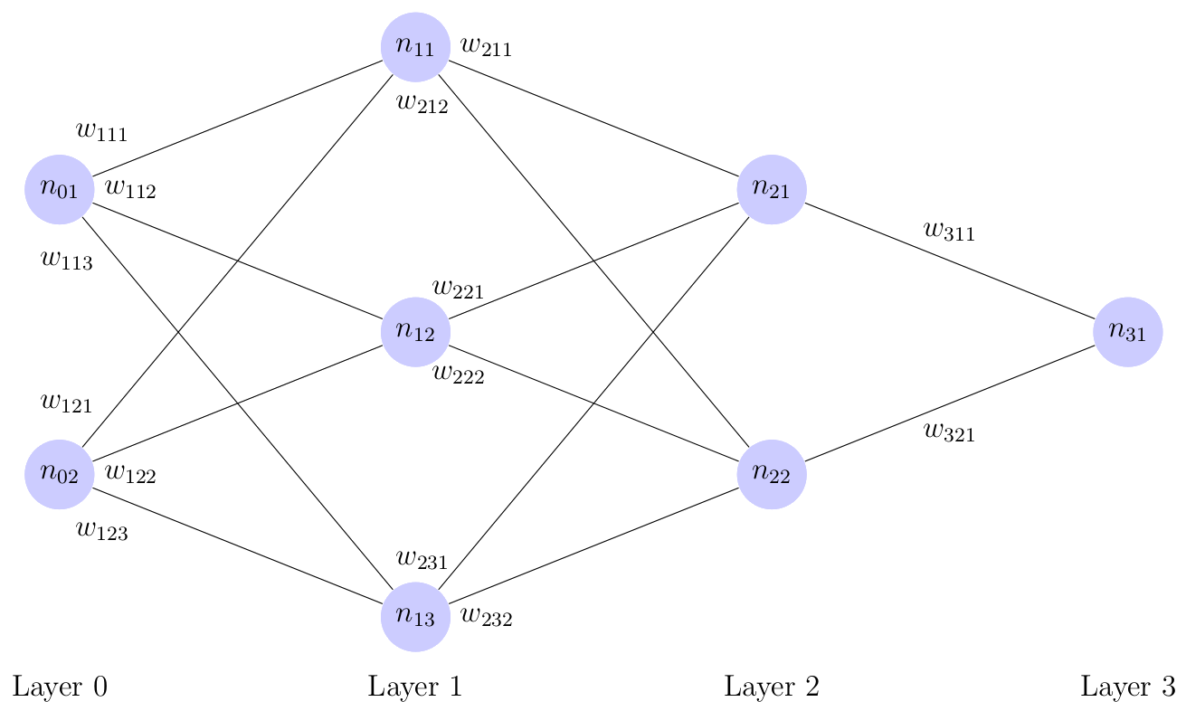
Figure 1: A Multi-Layer Perceptron Network
The input to a neuron \(n_{ij}\), also known as the "net" denoted \(\nu_{ij}\), is the weighted sum of all incoming edges plus an optional bias. Its output \(f_{i}(\nu_{ij})=o_{ij}\) is computed by applying the \(i\)-th layer's activation function \(f_{i}\) to \(\nu_{ij}\). By arranging the weights of each layer into a matrices , the output of the \(i\)-th layer of a MLP can be computed as:
\[\displaylines{\textbf{o}_{i}=f_{i}(\boldsymbol{\nu}_{i})=f_{i}(\textbf{W}_{i}^{T}\textbf{o}_{i-1}+\textbf{b}_{i})}\ .\]
where \(\boldsymbol{\nu}_{i}\) is vector of nets of the \(i\)-th layer, \(\textbf{W}_{i}\) is the weight matrix of the \(i\)-th layer, \(\textbf{b}_{i}\) is the bias vector of the \(i\)-th layer , and \(f_{i}(\textbf{x})\) is the activation function for the \(i\)-th layer. The activation function is applied component-wise to the resulting vector; \(tanh\) and the sigmoid function are commonly used. In a network with \(n+1\) layers, the final output \(\hat{\textbf{y}}\) given an input \(\textbf{x}\) can be defined as:
\[\displaylines{\hat{\textbf{y}}=\textbf{o}_{n}}\]
\[\displaylines{\textbf{o}_{i}= f_{i}(\textbf{W}_{i}^{T}\textbf{o}_{i-1}+\textbf{b}_{i})}\]
\[\displaylines{\textbf{o}_0=\textbf{x}}\ .\]
Back-Propagation
Consider a supervised learning scenario where the \(l\)-th input vector \(\textbf{x}^{(l)}\) is associated with the \(l\)-th target vector \(\textbf{y}^{(l)}\) with \(m\) input-target pairs in total. Further, assume the network has \(n+1\) layers of sizes: \(N_{0}, N_{1}, \ldots, N_{n}\). The L2 error of the network for this input at the \(i\)-th output neuron is then:\[\displaylines{E^{(l)}_{i}=\frac{1}{2}(\textbf{y}^{(l)}_{i}-\hat{\textbf{y}}^{(l)}_{i})^{2} }\ ,\]
where the \(1/2\) is for convenience, \(\textbf{y}^{(l)}_{i}\) is the \(i\)-th component of the target, and \(\hat{\textbf{y}}^{(l)}_{i}\) is the \(i\)-th component of the predicted output. The total network error is simply:
\[\displaylines{\sum\limits_{l=1}^{m}{E^{(l)}}=\sum\limits_{l=1}^{m}{\sum\limits_{i=1}^{N_n}{E^{(l)}_{i}}}=\sum\limits_{l=1}^{m}{\frac{1}{2}\lVert \textbf{y}^{(l)}-\hat{\textbf{y}}^{(l)} \rVert^{2}} }\ .\]
Back-propagation uses gradient descent to minimize the network error by updating the weights and biases of the network. First, consider the case of the output layer of the MLP network. After computing the network error for the \(l\)-th input sample, an update \(\Delta w_{ijk}^{(l)}\) is found for the entry in the \(j\)-th row and \(k\)-th column of the \(i\)-th weight matrix, that is \(w_{ijk}\). By the definition of gradient descent:
\[\displaylines{\Delta w_{ijk}^{(l)}=-\gamma \frac{\partial E_{k}^{(l)}}{\partial w_{ijk}} }\ ,\]
where \(\gamma\) is the learning rate. Now, by the multivariate chain rule,
\[\displaylines{\Delta w_{ijk}^{(l)}=-\gamma \frac{\partial E_{k}^{(l)}}{\partial w_{ijk}} = -\gamma \frac{\partial E_{k}^{(l)}}{\partial \nu_{ik}^{(l)}} \frac{\partial \nu_{ik}^{(l)}}{\partial w_{ijk}}}\]
\[\displaylines{= -\gamma \frac{\partial E_{k}^{(l)}}{\partial \nu_{ik}^{(l)}} o_{(i-1)j}^{(l)} }\ ,\]
where \(\nu_{ik}^{(l)}\) is the \(k\)-th neuron's net in the \(i\)-th layer of the network, and \(o_{(i-1)j}^{(l)}\) is the \(j\)-th neuron's output in layer \(i-1\) of the network. The final step is true since,
\[\displaylines{\boldsymbol{\nu}_{i}=\textbf{W}_{i}^{T}\textbf{o}_{i-1}+\textbf{b}_{i}}\ .\]
Only considering the \(k\)-th component of this, as above, results in:
\[\displaylines{\frac{\partial \nu_{ik}^{(l)}}{\partial w_{ijk}}= \frac{\partial }{\partial w_{ijk}}(w_{i1k}o_{(i-1)1}^{(l)}+\ldots+w_{ijk}o_{(i-1)j}^{(l)}+\ldots + w_{iN_{(i-1)}k}o_{(i-1)N_{(i-1)}}^{(l)})}\]
\[\displaylines{= o_{(i-1)j}^{(l)} }\ .\]
Continuing from earlier with the multivariate chain rule,
\[\displaylines{\frac{\partial E_{k}^{(l)}}{\partial \nu_{ik}^{(l)}} =\frac{\partial E_{k}^{(l)}}{\partial o_{ik}^{(l)}}\frac{\partial o_{ik}^{(l)}}{\partial \nu_{ik}^{(l)}} }\ .\]
Consider the case of the output layer, that is layer \(i=n\). Using the definition of the component-wise error defined earlier, the RHS simplifies as follows:
\[\displaylines{\frac{\partial E_{k}^{(l)}}{\partial o_{nk}^{(l)}}\frac{\partial o_{nk}^{(l)}}{\partial \nu_{nk}^{(l)}} = -2*\frac{1}{2}(\textbf{y}^{(l)}_{k}-o_{nk}^{(l)})\frac{\partial o_{nk}^{(l)}}{\partial \nu_{nk}^{(l)}}}\]
\[\displaylines{= (o_{nk}^{(l)}-\textbf{y}^{(l)}_{k})\frac{\partial f_{i}(\nu_{nk}^{(l)})}{\partial \nu_{nk}^{(l)}}=(o_{nk}^{(l)}-\textbf{y}^{(l)}_{k})f'_{i}(\nu_{nk}^{(l)})}\]
\[\displaylines{=(\hat{\textbf{y}}_{k}^{(l)}-\textbf{y}^{(l)}_{k})f'_{i}(\nu_{nk}^{(l)}) }\ .\]
If the activation function for a given layer is \(f_{i}=tanh\) then \(f'_{i}=1-f_{i}^{2}\) and thus can be easily computed. Thus, the update rule for output neurons is:
\[\displaylines{\Delta w_{njk}^{(l)}= - \gamma (\hat{\textbf{y}}_{k}^{(l)}-\textbf{y}^{(l)}_{k})f'_{i}(\nu_{nk}^{(l)}) o_{(n-1)j}^{(l)} }\]
\[\displaylines{= \gamma \delta_{nk}^{(l)} o_{(n-1)j}^{(l)} }\ ,\]
where \(\delta_{nk}^{(l)} = -\frac{\partial E_{k}^{(l)}}{\partial \nu_{nk}^{(l)}}\) is the \(k\)-th neuron's delta value in the output layer ( layer \(n\) of the MLP) for the \(l\)-th input vector.
For hidden layers, \(\frac{\partial E_{k}^{(l)}}{\partial o_{ik}^{(l)}}\) can no longer be directed computed as the target values \(\textbf{y}^{(l)}\) are only provided for the output layer. The delta terms for these layers are obtained through back-propagation. That is, the delta terms for layer \(i\) are obtained using those for layer \(i+1\) as can be seen below in Figure 2.
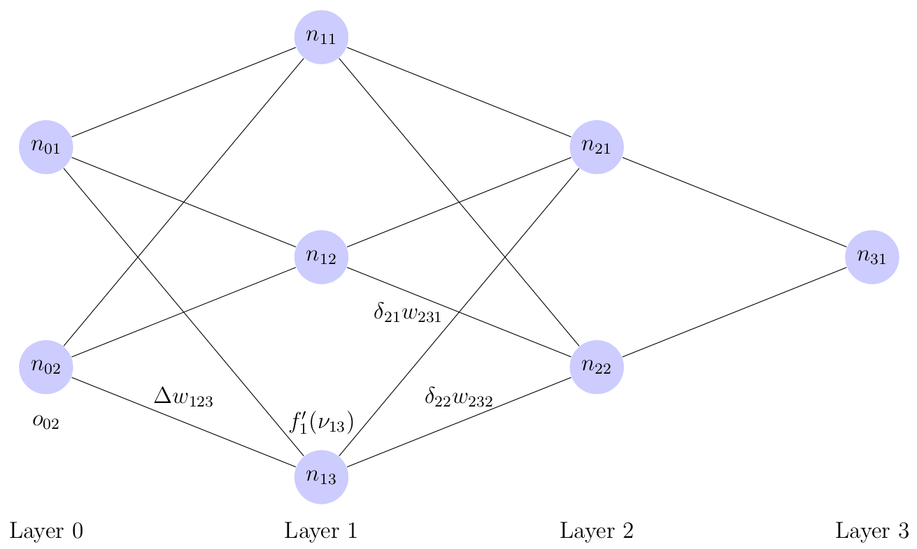
Figure 2: Hidden Node Update Visualization
One difference in the derivation between hidden nodes and output nodes is that, since the layers in MLP networks are fully-connected, hidden neurons contribute to the error in all later neurons. Thus, the total network error term \(E^{(l)}\) is used instead of the component-wise error \(E_{k}^{(l)}\). So, similar to above,
\[\displaylines{\Delta w_{ijk}^{(l)}=-\gamma \frac{\partial E^{(l)}}{\partial w_{ijk}} }\]
\[\displaylines{=-\gamma \frac{\partial E^{(l)}}{\partial \nu_{ik}^{(l)}} \frac{\partial \nu_{ik}^{(l)}}{\partial w_{ijk}}}\]
\[\displaylines{= -\gamma \frac{\partial E^{(l)}}{\partial \nu_{ik}^{(l)}} o_{(i-1)j}^{(l)}}\]
\[\displaylines{= -\gamma \frac{\partial E^{(l)}}{\partial o_{ik}^{(l)}}\frac{\partial o_{ij}^{(l)}}{\partial \nu_{ik}^{(l)}} o_{(i-1)j}^{(l)}}\]
\[\displaylines{= -\gamma \frac{\partial E^{(l)}}{\partial o_{ik}^{(l)}}f'_{i}(\nu_{ik}^{(l)}) o_{(i-1)j}^{(l)}}\ .\]
Next, replace the total network error by its earlier definition,
\[\displaylines{\Delta w_{ijk}^{(l)}= -\gamma \sum\limits_{c=1}^{N_i}{\frac{\partial E_{c}^{(l)}}{\partial o_{ik}^{(l)}}}f'_{i}(\nu_{ik}^{(l)}) o_{(i-1)j}^{(l)}}\]
\[\displaylines{= -\gamma \sum\limits_{c=1}^{N_i}{\frac{\partial E_{c}^{(l)}}{\partial \nu_{(i+1)c}^{(l)}}\frac{\partial \nu_{(i+1)c}^{(l)}}{\partial o_{ik}^{(l)}}}f'_{i}(\nu_{ik}^{(l)}) o_{(i-1)j}^{(l)}}\]
\[\displaylines{= \gamma \sum\limits_{c=1}^{N_i}{\delta_{(i+1)c}^{(l)} w_{(i+1)kc}} f'_{i}(\nu_{ik}^{(l)}) o_{(i-1)j}^{(l)}}\ .\]
The last step follows since the delta values for layer \(i+1\) have already been computed. Thus, in summary, the weight update is computed as
\[\displaylines{\Delta w_{ijk}^{(l)}= \gamma \delta_{ik}^{(l)} o_{(i-1)j}^{(l)} }\]
with
\[\displaylines{\delta_{ik}^{(l)} = (\textbf{y}^{(l)}_{k} - \hat{\textbf{y}}_{k}^{(l)})f'_{i}(\nu_{ik}^{(l)}) }\]
for output layers and
\[\displaylines{\delta_{ik}^{(l)} = \sum\limits_{c=1}^{N_i}{\delta_{(i+1)c}^{(l)} w_{(i+1)kc}} f'_{i}(\nu_{ik}^{(l)}) }\]
for hidden layers. In order to update bias weights, use the appropriate formula above and replace \(o_{(i-1)j}^{(l)}\) with 1.
Implementation in Python with NumPy
The above formulas can be conveniently implemented using matrix and component-wise multiplications of matrices.#bprop.py
#Author: nogilnick
import numpy as np
#Array of layer sizes
ls = np.array([2, 4, 4, 1])
n = len(ls)
#List of weight matrices (each a numpy array)
W = []
#Initialize weights to small random values
for i in range(n - 1):
W.append(np.random.randn(ls[i], ls[i + 1]) * 0.1)
#List of bias vectors initialized to small random values
B = []
for i in range(1, n):
B.append(np.random.randn(ls[i]) * 0.1)
#List of output vectors
O = []
for i in range(n):
O.append(np.zeros([ls[i]]))
#List of Delta vectors
D = []
for i in range(1, n):
D.append(np.zeros(ls[i]))
#Input vectors (1 row per each)
A = np.matrix([[0.0, 0.0], [0.0, 1.0], [1.0, 0.0], [1.0, 1.0]])
#Target Vectors (1 row per each)
y = np.matrix([[-0.5], [0.5], [0.5], [-0.5]])
#Activation function (tanh) for each layer
#Linear activation for final layer
actF = []
dF = []
for i in range(n - 1):
actF.append(lambda (x) : np.tanh(x))
#Derivative of activation function in terms of itself
dF.append(lambda (y) : 1 - np.square(y))
#Linear activation for final layer
actF.append(lambda (x): x)
dF.append(lambda (x) : np.ones(x.shape))
#Learning rate
a = 0.5
#Number of iterations
numIter = 250
#Loop for each iteration
for c in range(numIter):
#loop over all input vectors
for i in range(len(A)):
print(str(i))
#Target vector
t = y[i, :]
#Feed-forward step
O[0] = A[i, :]
for j in range(n - 1):
O[j + 1] = actF[j](np.dot(O[j], W[j]) + B[j])
print('Out:' + str(O[-1]))
#Compute output node delta values
D[-1] = np.multiply((t - O[-1]), dF[-1](O[-1]))
#Compute hidden node deltas
for j in range(n - 2, 0, -1):
D[j - 1] = np.multiply(np.dot(D[j], W[j].T), dF[j](O[j]))
#Perform weight and bias updates
for j in range(n - 1):
W[j] = W[j] + a * np.outer(O[j], D[j])
B[j] = B[j] + a * D[j]
print('\nFinal weights:')
#Display final weights
for i in range(n - 1):
print('Layer ' + str(i + 1) + ':\n' + str(W[i]) + '\n')In the above code, the delta values for each layer are computed simultaneously by using matrix multiplication instead of evaluating each component separately. Similarly, the weight updates are computed simultaneously using an outer product between the delta and output vectors.