Multi-Layer Perceptrons as Smoother Functions

Wed, 20 Apr 2016

Ann, Computer Science, Machine Learning, Mlp, Numpy, Python, Stock, Tensorflow

In this post, the multi-layer perceptron (MLP) is presented as a method for smoothing time series data. A class based on the TensorFlow library is presented. Finally, for the sake of a toy example, the class is applied to the problem of smoothing historical stock prices (*).

Data Setup

Yahoo Finance provides historical price data for a large number of stock tickers. In this post, historical price data for the ticker YHOO, over the period of April 1996 to April 2016, is retrieved from finance.yahoo.com. The file is in CSV format and consists of daily open, low, high, close and volume data for Yahoo Inc.

Update: YHOO is no longer traded; feel free to use the provided link or historical data from another company.

To pre-process the data for the neural network, the CSV file is loaded into Python using pandas. Specifically, the read_csv function is used. By providing the parse_dates argument, the Date column can be parsed and easily converted to a numerical value.

import pandas as pd

DF = pd.read_csv('yahoostock.csv', parse_dates=['Date'])
DF = DF.sort_values('Date')

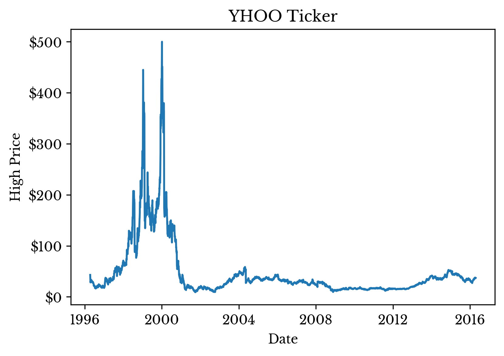
To demonstrate the use of smoother functions, only the market high for the day is preserved; the other columns are discarded. The high price for the day is plotted in Figure 1.

Figure 1: Daily Market High for the YHOO Ticker

Converting the datetime objects to integer values is accomplished using the astype method. As the datatype of the Date column is datetime64[ns], this call converts the column to the number of nanoseconds since January 1st 1970.

#y is the dependent variable
y = DF.High[:, None]
#A contains the independent variable
A  = DF.Date.astype('int')[:, None] * 1e-18

To reduce the magnitude of these values and improve overall numerical conditioning, the column is multiplied by 1e-18.

Creating the MLP

The MLP class that will be used follows a simple interface similar to that of the python scikit-learn library. The source code is available here. The interface is as follows:

#Fit the MLP to the data
#param A: numpy matrix where each row is a sample
#param y: numpy matrix of target values
def fit(self, A, y):

#Predict the output given the input (only run after calling fit)
#param A: The input values for which to predict outputs
#return: The predicted output values (one row per input sample)
def predict(self, A):

#Predicts the ouputs for input A and then computes the RMSE between
#The predicted values and the actualy values
#param A: The input values for which to predict outputs
#param y: The actual target values
#return: The RMSE
def score(self, A, y):

The first step is to create an artificial neural network regressor (ANNR) object. This can be done as follows:

#Number of neurons in the input layer
i = 1
#Number of neurons in the output layer
o = 1
#Number of neurons in the hidden layers
h = 32
#3 Fully-connected layers with tanh followed by linear output layer 
layers = [('F', h), ('AF', 'tanh'), ('F', h), ('AF', 'tanh'), ('F', h), ('AF', 'tanh'), ('F', o)]
mlpr = ANNR([i], layers, batchSize = 256, maxIter = 1000, tol = 0.2, reg = 1e-4, verbose = True)

With this code, an ANNR object will be initialized with the given layer sizes, a batch size of 256, a training iteration limit of 1000, an error tolerance of 0.20 (for the MSE), regularization weight of \(1e-4\), and verbose output enabled. The source code for the ANNR class shows how this is accomplished (see GitHub for the latest code).

#Create the MLP variables for TF graph
#_X: The input matrix
#_W: The weight matrices
#_B: The bias vectors
#_AF: The activation function
def _CreateMLP(_X, _W, _B, _AF):
    n = len(_W)
    for i in range(n - 1):
        _X = _AF(tf.matmul(_X, _W[i]) + _B[i])
    return tf.matmul(_X, _W[n - 1]) + _B[n - 1]

#Add L2 regularizers for the weight and bias matrices
#_W: The weight matrices
#_B: The bias matrices
#return: tensorflow variable representing l2 regularization cost
def _CreateL2Reg(_W, _B):
    n = len(_W)
    regularizers = tf.nn.l2_loss(_W[0]) + tf.nn.l2_loss(_B[0])
    for i in range(1, n):
        regularizers += tf.nn.l2_loss(_W[i]) + tf.nn.l2_loss(_B[i])
    return regularizers

#Create weight and bias vectors for an MLP
#layers: The number of neurons in each layer (including input and output)
#return: A tuple of lists of the weight and bias matrices respectively
def _CreateVars(layers):
    weight = []
    bias = []
    n = len(layers)
    for i in range(n - 1):
        #Fan-in for layer; used as standard dev
        lyrstd = np.sqrt(1.0 / layers[i])
        curW = tf.Variable(tf.random_normal([layers[i], layers[i + 1]], stddev = lyrstd))
        weight.append(curW)
        curB = tf.Variable(tf.random_normal([layers[i + 1]], stddev = lyrstd))
        bias.append(curB)
    return (weight, bias)

...

#The constructor
#param layers: A list of layer sizes
#param actvFn: The activation function to use: 'tanh', 'sig', or 'relu'
#param learnRate: The learning rate parameter
#param decay: The decay parameter
#param maxItr: Maximum number of training iterations
#param tol: Maximum error tolerated
#param batchSize: Size of training batches to use (use all if None)
#param verbose: Print training information
#param reg: Regularization weight
def __init__(self, layers, actvFn = 'tanh', learnRate = 0.001, decay = 0.9, maxItr = 2000,
             tol = 1e-2, batchSize = None, verbose = False, reg = 0.001):
    #Parameters
    self.tol = tol
    self.mItr = maxItr
    self.vrbse = verbose
    self.batSz = batchSize
    #Input size
    self.x = tf.placeholder("float", [None, layers[0]])
    #Output size
    self.y = tf.placeholder("float", [None, layers[-1]])
    #Setup the weight and bias variables
    weight, bias = _CreateVars(layers)
    #Create the tensorflow MLP model
    self.pred = _CreateMLP(self.x, weight, bias, _GetActvFn(actvFn))
    #Use L2 as the cost function
    self.loss = tf.reduce_sum(tf.nn.l2_loss(self.pred - self.y))
    #Use regularization to prevent over-fitting
    if(reg is not None):
        self.loss += _CreateL2Reg(weight, bias) * reg
    #Use ADAM method to minimize the loss function
    self.optmzr = tf.train.AdamOptimizer(learning_rate=learnRate).minimize(self.loss)

As seen above, tensorflow placeholder variables are created for the input (x) and the output (y). Next, tensorflow variables for the weight matrices and bias vectors are created using the _CreateVars() function. The weights are initialized as random normal numbers distributed as \(\mathcal{N}(0, 1/\sqrt{f})\), where \(f\) is the fan-in to the layer.

Next, the MLP model is constructed using its definition as discussed in an earlier post. After that, the loss and regularization functions are defined as the L2 loss. Regularization penalizes larger values in the weight matrices and bias vectors to help prevent over-fitting. Lastly, tensorflow's AdamOptimizer is employed as the training optimizer with the goal of minimizing the loss function. Note that at this stage the learning has not yet been done, only the tensorflow graph has been initialized with the necessary components of the MLP.

Next, the MLP is trained with the Yahoo stock data. A hold-out period is used to assess how well the MLP is performing. This can be accomplished as follows:

#Length of the hold-out period
nDays = 5
n = len(A)
#Learn the data
mlpr.fit(A[0:(n-nDays)], y[0:(n-nDays)])

When the fit function is called, the actual training process begins. First, a tensorflow session must be created and all variables defined in the constructor must be initialized. Then, training iterations are performed up to the iteration limit provided, the weights are updated, and the error is recorded. The feed_dict parameter specifies the values of our inputs (x) and outputs (y). If the error falls below the tolerance level, training is completed, otherwise the maximum number of iterations is exhausted.

#Fit the MLP to the data
#param A: numpy matrix where each row is a sample
#param y: numpy matrix of target values
def fit(self, A, y):
    m = len(A)
    #Start the tensorflow session and initializer
    #all variables
    self.sess = tf.Session()
    init = tf.initialize_all_variables()
    self.sess.run(init)
    #Begin training
    for i in range(self.mItr):
        #Batch mode or all at once
        if self.batSz is None:
            self.sess.run(self.optmzr, feed_dict={self.x:A, self.y:y})
        else:
            for j in range(0, m, self.batSz):
                batA, batY = _NextBatch(A, y, j, self.batSz)
                self.sess.run(self.optmzr, feed_dict={self.x:batA, self.y:batY})
        err = self.sess.run(self.loss, feed_dict={self.x:A, self.y:y})
        err = np.sqrt(err * 2.0 / m)
        if self.vrbse:
            print('Iter {:6d} {:f}'.format(i + 1, err))
        if self.tol > err:
            break

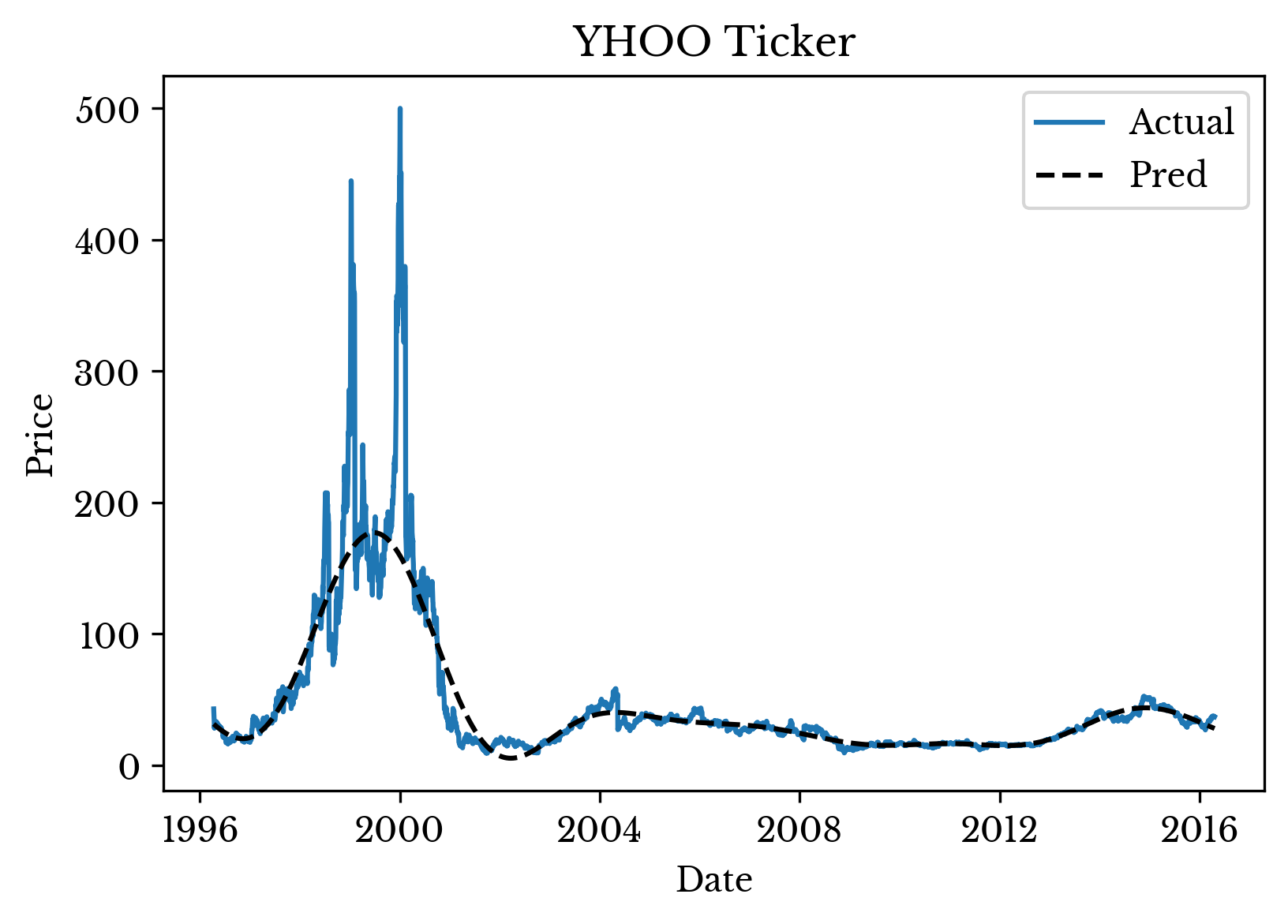
With the MLP network trained, prediction is performed and results are plotted using matplotlib. Figure 3 shows the smoothed curve superimposed over the original data.

Figure 2: Actual and Smoothed Time Series Data

As can be seen, the MLP smooths the original stock data. The amount of smoothing is dependent upon the MLP parameters including the number of layers, the size of the layers, the error tolerance, and the amount of regularization. Neural networks feature a relatively large number of hyper-parameters and a significant amount of tuning is frequently required to achieve satisfactory results.

Note (*): The contents of this post are for educational purposes only. The contents are not intended to be used to devise a trading strategy and do not constitute financial advice. Financial markets are exceedingly complex and a naive approach such as the above is likely no better than random guessing.