Decorrelating Features using the Gram-Schmidt Process

Thu, 04 Oct 2018

Data Science, Linear Algebra, Linear Models, Machine Learning, Mathematics, Statistics

A problem that frequently arises when applying linear models is that of multicollinearity. The term multicollinearity describes the phenomenon where one or more features in the data matrix can be accurately predicted using a linear model involving others of the features. The consequences of multicollinearity include numerical instability due to ill-conditioning, and difficulty in interpreting the regression coefficients. An approach to decorrelate features is presented using the Gram-Schmidt process.

The Gram-Schmidt Process

The Gram-Schmidt process is typically presented as a process for orthonormalizing the columns of a matrix. Let \(\textbf{A}\) be an m x n matrix with each row being a sample and each column a feature. Further, define \(\textbf{B}\) as the transformed matrix and \(\textbf{X}_{i}\) as the i-th column of a matrix \(\textbf{X}\). Using this notation, the orthonormalized matrix \(\textbf{B}\) is computed as

\[\displaylines{\textbf{B}^{*}_{i} = \textbf{A}_{i} - \sum\limits_{j=1}^{i-1}{P(\textbf{B}^{*}_{j}, \textbf{A}_{i})}\\ \textbf{B}_{i}=\frac{\textbf{B}^{*}_{i}}{||\textbf{B}^{*}_{i}||}}\] for \[\displaylines{i = 1,2,\ldots,n}\ ,\]

where,

\[\displaylines{P(\textbf{u}, \textbf{v}) = \frac{\langle \textbf{u},\textbf{v}\rangle}{\langle \textbf{u},\textbf{u}\rangle}\textbf{u} }\]

is the projection of v onto u, and \(\langle \textbf{u},\textbf{v}\rangle\) denotes the inner product of these vectors

The Gram-Schmidt process accomplishes orthonormalization when the dot product is used as the inner-product. Recall that the dot-product of two vectors is defined as:

\[\displaylines{\textbf{x} \cdot \textbf{y} = \sum\limits_{i=1}^{n}{x_{i}y_{i}}}\]

If the dot product of two vectors x and y is 0, then the vectors are orthogonal to each-other. This implies that the angle between the two vectors is 90°. After performing the Gram-Schmidt process, the inner-product of any pair of columns in the transformed matrix is 0. Thus, the resulting matrix is orthogonal.

Covariance and Inner Products

The Gram-Schmidt process does not require that the dot product be used as inner-product in \(P(\textbf{u}, \textbf{v})\). In this case, the goal is to decorrelate the columns of the matrix A not to make them orthogonal. This can be accomplished using the same procedure with an appropriate operator as inner product. In this case, the operator that is considered is covariance. Define

\[\displaylines{C(\textbf{x}, \textbf{y})=\frac{1}{2n^{2}}\sum\limits_{i=1}^{n}\sum\limits_{j=1}^{n}{(x_i-x_j)(y_i-y_j)} }\]

as the covariance of the vectors x and y. The above definition is used for convenience despite being more inefficient than the typical definition using the vector means.

In order for an operator to be defined as an inner product, it must satisfy four criteria.

\(\langle \textbf{u},\textbf{v}\rangle = \langle \textbf{v},\textbf{u}\rangle\)
\(\langle a\textbf{u},\textbf{v}\rangle = a\langle \textbf{u},\textbf{v}\rangle\)
\(\langle \textbf{u}+\textbf{w},\textbf{v}\rangle = \langle \textbf{u},\textbf{v}\rangle + \langle \textbf{w},\textbf{v}\rangle\)
\(\langle \textbf{u},\textbf{u}\rangle \geq 0\) and \(\langle \textbf{u},\textbf{u}\rangle = 0\) iff \(\textbf{u} = 0\)

Criteria 1

\[\displaylines{C(\textbf{x}, \textbf{y})=\frac{1}{2n^{2}}\sum\limits_{i=1}^{n}\sum\limits_{j=1}^{n}{(x_i-x_j)(y_i-y_j)} \\ = \frac{1}{2n^{2}}\sum\limits_{i=1}^{n}\sum\limits_{j=1}^{n}{(y_i-y_j)(x_i-x_j)} \\ = C(\textbf{y}, \textbf{x})}\]

Criteria 2

\[\displaylines{C(a\textbf{x}, \textbf{y})=\frac{1}{2n^{2}}\sum\limits_{i=1}^{n}\sum\limits_{j=1}^{n}{(ax_i-ax_j)(y_i-y_j)} \\ = \frac{1}{2n^{2}}\sum\limits_{i=1}^{n}\sum\limits_{j=1}^{n}{a(x_i-x_j)(y_i-y_j)} \\ = a \times C(\textbf{x}, \textbf{y})}\]

Criteria 3

\[\displaylines{C(\textbf{x}+\textbf{z}, \textbf{y})=\frac{1}{2n^{2}}\sum\limits_{i=1}^{n}\sum\limits_{j=1}^{n}{((x_i+z_i)-(x_j+z_j))(y_i-y_j)} \\ = \frac{1}{2n^{2}}\sum\limits_{i=1}^{n}\sum\limits_{j=1}^{n}{[(x_i-x_j)+(z_i-z_j)](y_i-y_j)} \\ = \frac{1}{2n^{2}}\sum\limits_{i=1}^{n}\sum\limits_{j=1}^{n}{[(x_i-x_j)(y_i-y_j)+(z_i-z_j)(y_i-y_j)]} \\ = \frac{1}{2n^{2}}\sum\limits_{i=1}^{n}\sum\limits_{j=1}^{n}{(x_i-x_j)(y_i-y_j)}+\frac{1}{2n^{2}}\sum\limits_{i=1}^{n}\sum\limits_{j=1}^{n}{(y_i-y_j)(z_i-z_j)} \\ = C(\textbf{x}, \textbf{y}) + C(\textbf{y}, \textbf{z})}\]

Criteria 4

\[\displaylines{C(\textbf{x}, \textbf{x})=\frac{1}{2n^{2}}\sum\limits_{i=1}^{n}\sum\limits_{j=1}^{n}{(x_i-x_j)(x_i-x_j)} \\ = \frac{1}{2n^{2}}\sum\limits_{i=1}^{n}\sum\limits_{j=1}^{n}{(x_i-x_j)^2}\geq 0 }\]

Unfortunately, this fourth condition is only partially true. The covariance of any constant vector is 0 and so the vector being 0 is a sufficient but not a necessary condition. Thus, covariance is positive semi-definite and not positive-definite as required.

By carefully restricting the subspace of vectors, this condition can be made true in the reduced space. If the features are assumed to have mean 0, this condition holds. Intuitively, any constant vector that is mean centered becomes the 0 vector.

It can be shown that this construction is valid using the concept of quotient vector spaces. Instead of considering the space of all random variables, a quotient space is constructed in which all random variables that differ by only a constant are identified. In this quotient space, covariance is a true inner product. Further, the space of mean centered vectors is isomorphic to this quotient space.

Since it is assumed that the vectors are centered, only centered vectors must be used throughout the Gram-Schmidt process. A short proof follows which shows that all vectors produced in the intermediate steps of the process are centered.

Lemma:

If \[\displaylines{\bar{\textbf{A}}_{i}=0 }\] for \[\displaylines{i = 1,2,\ldots,n}\]

Then \[\displaylines{\bar{\textbf{B}}_{i}=0 }\] for \[\displaylines{i = 1,2,\ldots,n}\ .\]

Proof: By definition, \(\textbf{B}^{*}_{0}=\textbf{A}_{0}\) is centered, since \(\textbf{A}_{0}\) is centered. The proof proceeds using mathematical induction. Using the definition of \(\textbf{B}_{i}\) and the mean,

\[\displaylines{\textbf{B}_{i} = (\textbf{A}_{i} - \sum\limits_{j=1}^{i-1}{\frac{\langle \textbf{B}^{*}_{j}, \textbf{A}_{i} \rangle}{\langle \textbf{A}_{i}, \textbf{A}_{i} \rangle}\textbf{B}^{*}_{j}})/||\textbf{B}^{*}_{i}|| }\ ,\]

and so,

\[\displaylines{\bar{\textbf{B}}_{i} = (\frac{1}{m}\sum\limits_{k=1}^{m}{(\textbf{A}_{ki} - \sum\limits_{j=1}^{i-1}{\frac{\langle \textbf{B}^{*}_{j}, \textbf{A}_{i} \rangle}{\langle \textbf{A}_{i}, \textbf{A}_{i} \rangle}\textbf{B}^{*}_{kj}})})/||\textbf{B}^{*}_{i}||\\ = \frac{1}{||\textbf{B}^{*}_{i}||}\frac{1}{m}\sum\limits_{k=1}^{m}{\textbf{A}_{ki}} - \frac{1}{||\textbf{B}^{*}_{i}||}\frac{1}{m}\sum\limits_{k=1}^{m}{\sum\limits_{j=1}^{i-1}{\frac{\langle \textbf{B}^{*}_{j}, \textbf{A}_{i} \rangle}{\langle \textbf{A}_{i}, \textbf{A}_{i} \rangle}\textbf{B}^{*}_{kj}}}\\ = 0 - \frac{1}{||\textbf{B}^{*}_{i}||}\frac{\langle \textbf{B}^{*}_{j}, \textbf{A}_{i} \rangle}{\langle \textbf{A}_{i}, \textbf{A}_{i} \rangle}\sum\limits_{j=1}^{i-1}{\frac{1}{m}\sum\limits_{k=1}^{m}{\textbf{B}^{*}_{kj}}}\\ = 0 - \frac{1}{||\textbf{B}^{*}_{i}||}\frac{\langle \textbf{B}^{*}_{j}, \textbf{A}_{i} \rangle}{\langle \textbf{A}_{i}, \textbf{A}_{i} \rangle}\sum\limits_{j=1}^{i-1}{\bar{\textbf{B}}^{*}_{j}}\\ = 0 - 0 = 0 }\ .\]

In the above, \(\bar{\textbf{A}}_{i}\) indicates the mean of column \(\textbf{A}_{i}\) and \(\textbf{A}_{ki}\) indicates the element in the k-th row and i-th column of the matrix \(\textbf{A}\).In the final step, the induction hypothesis, that \(\bar{\textbf{B}}^{*}_{j}=0\) for \(j<i\), is used. Thus, if the data matrix is centered, the Gram-Schmidt process only operates on centered vectors; the assumption remains valid throughout the process.

The Decorrelation Procedure

To proceed, the data matrix \(\textbf{A}\) is standardized. This fulfills the condition required above and causes the covariance of columns in the standardized matrix to be equal to the correlation. Recall that the Pearson correlation coefficient is defined as

\[\displaylines{R(\textbf{x}, \textbf{y})=\frac{C(\textbf{x},\textbf{y})}{\sigma_{\textbf{x}}\sigma_{\textbf{y}}} }\]

Where \(\sigma_{\textbf{x}}\) is the standard deviation of x. Thus, the correlation and covariance are equal in this case, since the standardized columns have variance one.

Next the Gram-Schmidt process is applied sequentially on the columns. The first column is left unchanged since it already has variance 1. The second transformed column is computed as the second original column with any portion that is correlated to first column removed. In general, the i-th transformed column is equal to the i-th original column with any portion that is linearly correlated to the j-th transformed column removed for all \(j<i\).

An Example

An example is presented using the automobile MPG dataset available from UCI. The dataset is used to train a model which can predict city-cycle fuel economy given several numerical and categorical features. Only the numerical features are considered here.

	Weight	Displacement	Cylinders	Acceleration
Cylinders	1.00	0.93	0.90	-0.42
Displacement	0.93	1.00	0.95	-0.54
Weight	0.90	0.95	1.00	-0.51
Acceleration	-0.42	-0.54	-0.51	1.00

Table 1: Auto MPG Feature Correlation

The correlation between the variables can easily be computed using pandas: A.corr(). The resulting correlation matrix shown in Table 1.

def Cov(X, Y):
   return ((X - X.mean()) * (Y - Y.mean())).mean()

def Proj(X, Y, F=Cov):
   return X * (F(X, Y) / F(X, X))

def ToUnit(X, F=Cov):
   return X / np.sqrt(F(X, X))

def GramSchmidt(A, F=Cov):
   B = A.copy()
   n = A.shape[1]
   for i in range(n):
      for j in range(i):
         B[:, i] = B[:, i] - Proj(B[:, j], B[:, i], F=F)
      B[:, i] = ToUnit(B[:, i], F=F)
   return B

The \(R^2\) of a linear regression model fit to the data is 0.7007. Next the method described above is implemented and the data matrix is transformed.

	Weight	Displacement	Cylinders	Acceleration
Weight	1.00	0.00	0.00	0.00
Displacement	0.00	1.00	0.00	0.00
Cylinders	0.00	0.00	1.00	0.00
Acceleration	0.00	0.00	0.00	1.00

Table 2: Transformed Auto MPG Feature Correlation

The resulting correlation matrix is shown in Table 2. Note that the correlation matrix is diagonal indicating that there is no correlation between the columns. The Gram-Schmidt process successfully decorrelated the data matrix! Figures 1 and 2 show scatter charts of MPG against the four features before and after decorrelation respectively.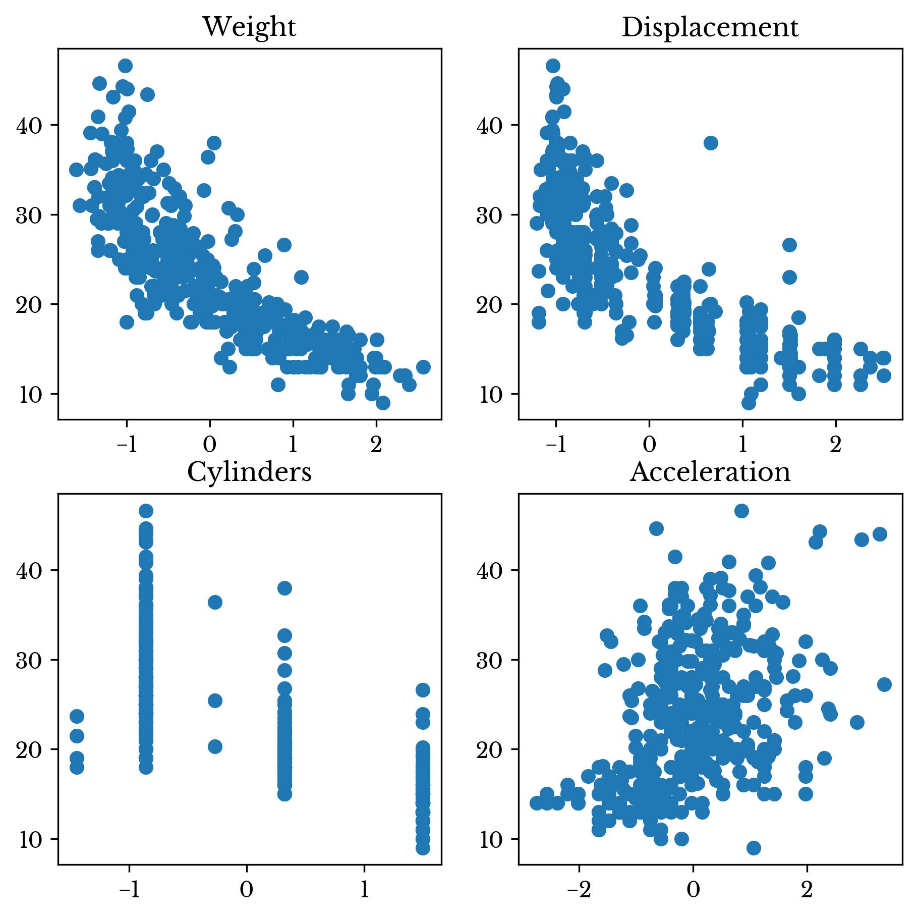

Figure 1: Scatter Plots of Original Data Against MPG

A linear regression model fit on the decorrelated data matrix achieves the same \(R^2\) of 0.7007. Further of interest is that the univariate regression coefficients for each column exactly match the multivariate coefficients of the full decorrelated matrix. Also, the sum of the univariate \(R^2\) values equal the multivariate regression \(R^2\). The above are both due to the columns having no linear correlation to each other.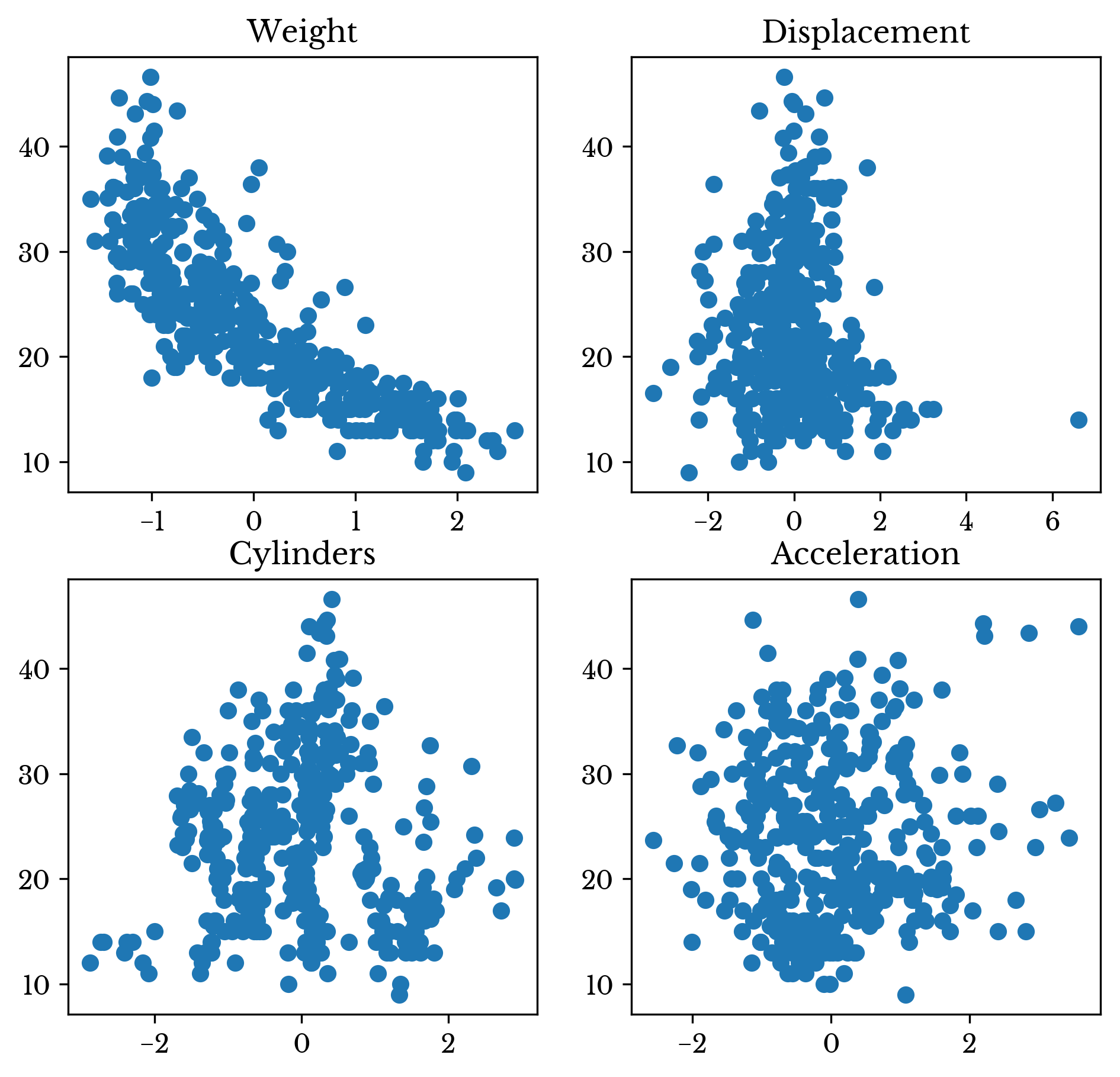

Figure 2: Scatter Plots of Decorrelated Data Against MPG

As can be seen in Table 3, the sum of the \(R^2\) values for the original features is inflated as some variables explain the same variation in MPG.

Feature	Orig. R²	Tran. R²
Weight	0.69179	0.69179
Displacement	0.64674	0.00618
Cylinders	0.60124	0.00027
Acceleration	0.17664	0.00245
Total	2.11642	0.70070

Table 3: Transformed Auto MPG Feature Correlation

While the multivariate and univariate regression coefficients are identical for the decorrelated data, the intercepts are different. However, the multivariate intercept can be derived from the univariate intercepts using the following formula.

\[\displaylines{b^{*}=\sum\limits_{i=1}^{n}{{b_i}-(n-1)\bar{Y}} }\]

Where \(b^{*}\) is the multivariate intercept, \(b_i\) is the i-th univariate regression coefficient, \(n\) is the number of columns in the data matrix, and \(\bar{Y}\) is the mean target value.

Conclusion

Principal component analysis also produces an uncorrelated transformed matrix. However, due to the nature of the transform, it is difficult to interpret the projected vectors. The aim of this post is to present a method that can be used to decorrelate a data matrix suffering from multicollinearity in a way that is more transparent. In this case, a transformed column has had all portions that are linearly correlated to the previous columns removed.

As seen in the example provided, this method does not improve the \(R^2\) of the model. Instead, the method is presented as a way of aiding the introspection of linear models on highly collinear data sets.

Note: See Decorrelation Redux to read about another approach to decorrelating the columns of a matrix that leverages the Cholesky decomposition.