Using Random Forests and Wordclouds to Visualize Feature Importance in Document Classification

Thu, 17 Aug 2017

Computer Science, Data Science, Data Visualization, Machine Learning, Matplotlib, Nlp, Python, Random Forest, Wordcloud

What characteristics do the works of famous authors have that make them unique? This post uses ensemble methods and wordclouds to explore just that.

Introduction

Project Gutenberg offers a large number of freely available works from many famous authors. The dataset for this post consists of books, taken from Project Gutenberg, written by each of the following authors:

Austen
Dickens
Dostoyevsky
Doyle
Dumas
Stevenson
Stoker
Tolstoy
Twain
Wells

The main idea of this post is to do the following:

Use vectors of word frequencies as features
Fit a random forest classifier for each author
Analyze each random forest to determine important features
Obtain words that correspond to important features
Create a word cloud with word size determined by importance

Data Setup

A number of libraries are necessary for this post.

import numpy as np
import matplotlib as mpl
from sklearn.feature_extraction.text import TfidfVectorizer, ENGLISH_STOP_WORDS
from sklearn.ensemble import RandomForestClassifier
from sklearn.feature_selection import SelectKBest
from nltk.corpus import wordnet as wn
import os
import roman
from PIL import Image
from wordcloud import WordCloud
from treeinterpreter import treeinterpreter as ti

The books for each author are organized in the following structure:

Austen/
    Book1.txt
    Book2.txt
    Book3.txt
    Book4.txt
Dickens/
    Book1.txt
...

The following code loads the books into memory. A number of strings are randomly generated from each book to increase the total number of samples. This prevents trees in the random forest from having height 0; a case which is not handled correctly in the treeinterpreter library. A potential fix for this which eliminates the need for sampling can be found here.

#%% Generate samples from each book
NWORDS = 2 ** 15
A = ['Austen', 'Dickens', 'Dostoyevsky', 'Doyle',
     'Dumas', 'Stevenson', 'Stoker', 'Tolstoy',
     'Twain', 'Wells']
tp = r"(?u)\b\w{2,}\b"                                      #Regex for words
ctp = re.compile(tp)
SW = GetSW()    #Stop words
BT = []         #List of randomly generated strings
AL = []         #Author labels
W = set()       #Big set of all words
for i, AFi in enumerate(A):
    for b in os.listdir(AFi):
        with open(os.path.join(AFi, b)) as F:
            ST = ctp.findall(F.read().lower())              #Tokenize book
        nSamp = np.ceil(len(ST) / NWORDS).astype(int)       #Number of samples
        for Ri in np.random.choice(ST, (nSamp, NWORDS)):    #Generate samples from book
            BT.append(' '.join(Ri))                         #Form string from sample
            W.update(Ri)                                    #Add any new words to vocabulary
            AL.append(AFi)                                  #Class label for this sample
#%% Form the vocabulary for Tfidf by removing invalid words/names/etc
def WordFilter(W):
    return (W in SW) or (len(wn.synsets(W)) == 0)

W = frozenset(Wi for Wi in W if not WordFilter(Wi))
AL = np.array(AL)

The WordFilter function utilizes wordnet to filter any invalid words. Wordnet is a very powerful library that can be used to analyze the meaning of natural language. For this code, wordnet is being used like a dictionary; if no entry is found for word W then W is filtered.

Tfidf Feature Extraction

The next step is to extract numerical features from the strings. For this, a TfidfVectorizer is used. Tfidf stands for: Term Frequency (times) Inverse Document Frequency. In math notation, Tfidf features are computed as

\(tf(t, d) \times idf(t)\) ,

where \(t\) is the term (a word in this case), \(d\) is the document (a randomly generated string), and \(tf\) is a function which counts the number of occurences of \(t\) in \(d\). The \(idf\) function is computed as

\(\log{\frac{1+n_{d}}{1+df(d, t)}}+1\) ,

where \(n_{d}\) is the total number of documents and \(df(t)\) is the number of documents that contain \(t\).

The \(idf(t)\) element aims to reduce the weight of terms which are common to all or most documents. With Tfidf features, idf(t) typically reduces the weight of \(tf(t, d)\) for terms like a, an, he, and she to prevent these terms from dwarfing more useful ones.

The following code computes tfidf features using sklearn.

#%% Transform text into numerical features
cv = TfidfVectorizer(token_pattern = tp, vocabulary = W)
TM = cv.fit_transform(BT)
#Lookup word by column index
IV = np.zeros((len(cv.vocabulary_)), dtype = object)
for k, v in cv.vocabulary_.items():
    IV[v] = k

Classification using Random Forest

Next, a binary random forest classifier is fit for each author; each classifier determines if a document is sampled from the works of a certain author or it is not. A random forest consists of a collection of decision trees (hence forest). An example of a random forest having 2 decision trees is shown below in Figure 1.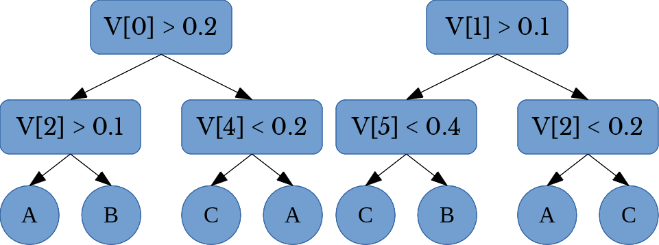

Figure 1: A Random Forest with 2 Trees

In the above figure, \(V[i]\) denotes the \(i\)-th element of the feature vector. The random forest depicted in Figure 1 predicts one of 3 class labels: A, B, or C.

A random forest with \(n\) trees is created by forming \(n\) random samples of size \(m\) from the training data. In this case, each set of random samples consists of \(m\) randomly selected rows of the data matrix TM. For each set, a decision tree is fit. A random forest performs classification by using a voting method. Each tree in the forest produces a class label and the class label that appears most is taken as the final prediction.

With a random forest fit to the training data, treeinterpreter is used to obtain the contribution of each feature in determining the predicted class label for each sample. The following code fits a random forest for each author and produces a dictionary which maps words to their importance. Note: It seems treeinterpreter does not use sparse features, so the amount of memory used in this snippet increases greatly with the number of trees in the random forest (n_estimators). Based on the amount of memory available, the number of trees and the number rows to predict per iteration can be adjusted.

#%%
def SplitArr(n, m):
    i1, i2 = 0, n % m if (n % m != 0) else m
    while i1 < n:
        yield i1, i2
        i1, i2 = i2, i2 + m
        
AW = []
for i, Ai in enumerate(A):
    #Use boolean class labels
    L = AL == Ai
    #Use an RFC to find most important words for each author
    C = RandomForestClassifier(n_estimators = 256, n_jobs = -1)
    C.fit(TM, L)
    S1 = C.score(TM, L)
    print('Accuracy {:10s}: {:.4f}'.format(Ai, S1))
    #Index of author class
    ACI = C.classes_.nonzero()[0][0]
    FR = csr_matrix((1, TM.shape[1]))
    #Iterate over rows in chunks to prevent out of memory
    NZR = L.nonzero()[0]
    for j1, j2 in SplitArr(len(NZR), 2):
        _, _, F = ti.predict(C, TM[j1:j2])
        FR += csr_matrix(F[:, :, ACI].sum(axis = 0))
    FR /= L.sum()
    AW.append({IV[j]: FR[0, j] for j in FR.nonzero()[1]})

Good results can also be obtained by using other feature selections techniques. SelectKBest from the feature_extraction module of sklearn, in particular, gives good results and is very efficient on sparse features. Code to use SelectKBest follows.

AW = []
for i, Ai in enumerate(A):
    L = AL == Ai
    C = SelectKBest(k = 1024)
    C.fit(TM, L)
    FR = C.scores_
    AW.append({IV[j]: FR[j] for j in FR.nonzero()[0]})

Visualization of Features using Wordclouds

AW now contains a dictionary of words mapped to their importance for each author. Next, a wordcloud is constructed using the wordcloud library. The generate_from_frequencies function allows a wordcloud to be constructed from a dictionary. Transparency masks are also used so that the words are filled into a pattern specified by the mask parameter.

cmi = 0
def MakeCF():
    global cmi
    CM = [mpl.cm.Greens, mpl.cm.Oranges, mpl.cm.Blues][cmi % 3]
    cmi += 1
    def color_func(word, font_size, position, orientation, random_state=None, **kwargs):
        return tuple(int(255 * j) for j in CM(np.random.rand() + .4))
    return color_func
    
#%% Create wordclouds
fontPath = 'C:\\Windows\\Fonts\\SpecialElite.ttf'
for i, Ai in enumerate(A):
    icon = Image.open(os.path.join('Masks', Ai + '.png'))
    mask = Image.new("RGB", icon.size, (255, 255, 255))
    mask.paste(icon, icon)
    mask = np.array(mask)
    wc = WordCloud(background_color = None, color_func = MakeCF(), 
         font_path = fontPath, mask = mask, max_font_size = 250, mode = 'RGBA')            
    wc.generate_from_frequencies(AW[i])
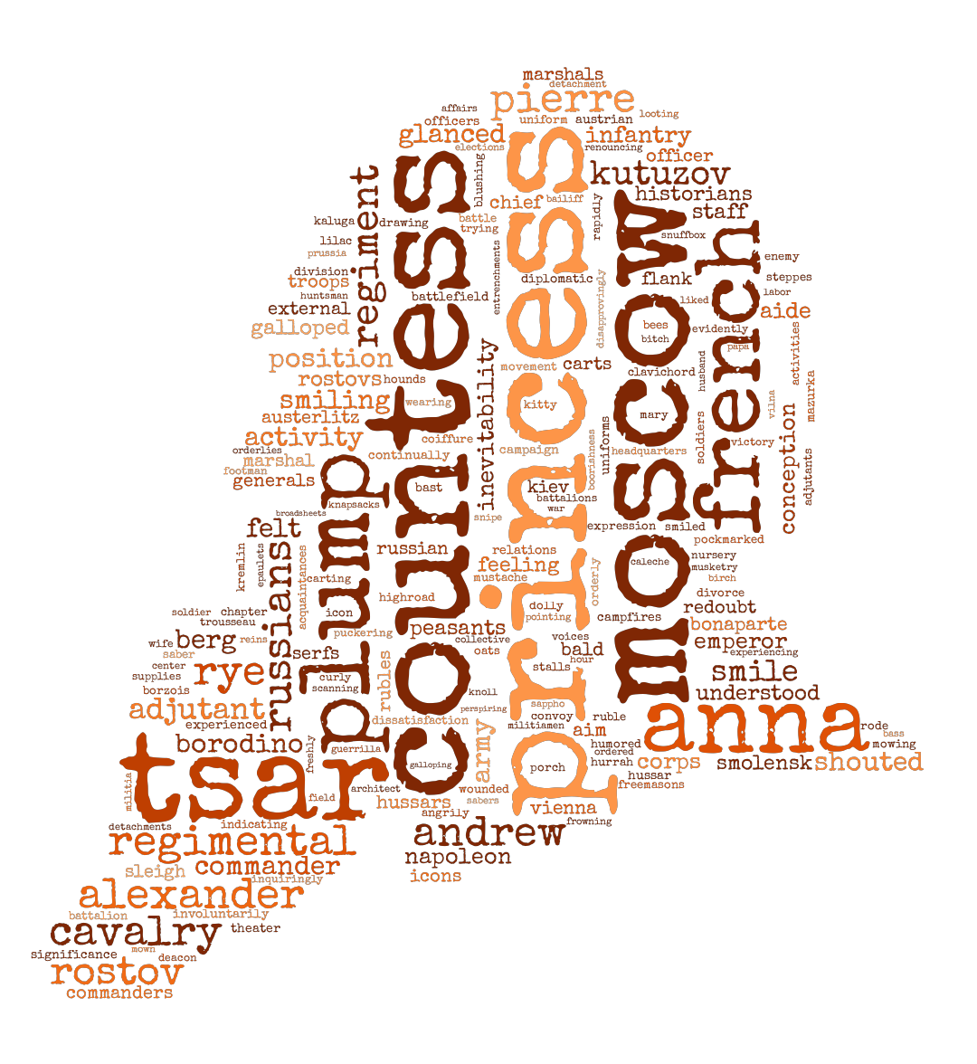
    wc.to_file(os.path.join('Wordclouds', Ai + '.png'))

In the above code, the word color is randomly chosen using colormaps from MatPlotLib. The font used is a Google Font called: Special Elite. The font is available for download here. The resulting wordclouds are shown below in Figures 2 and 3.

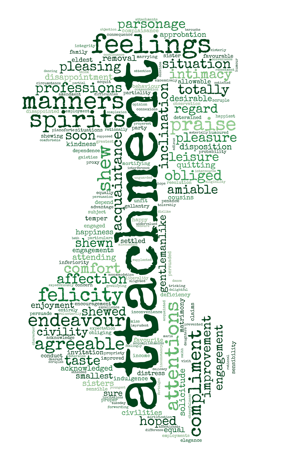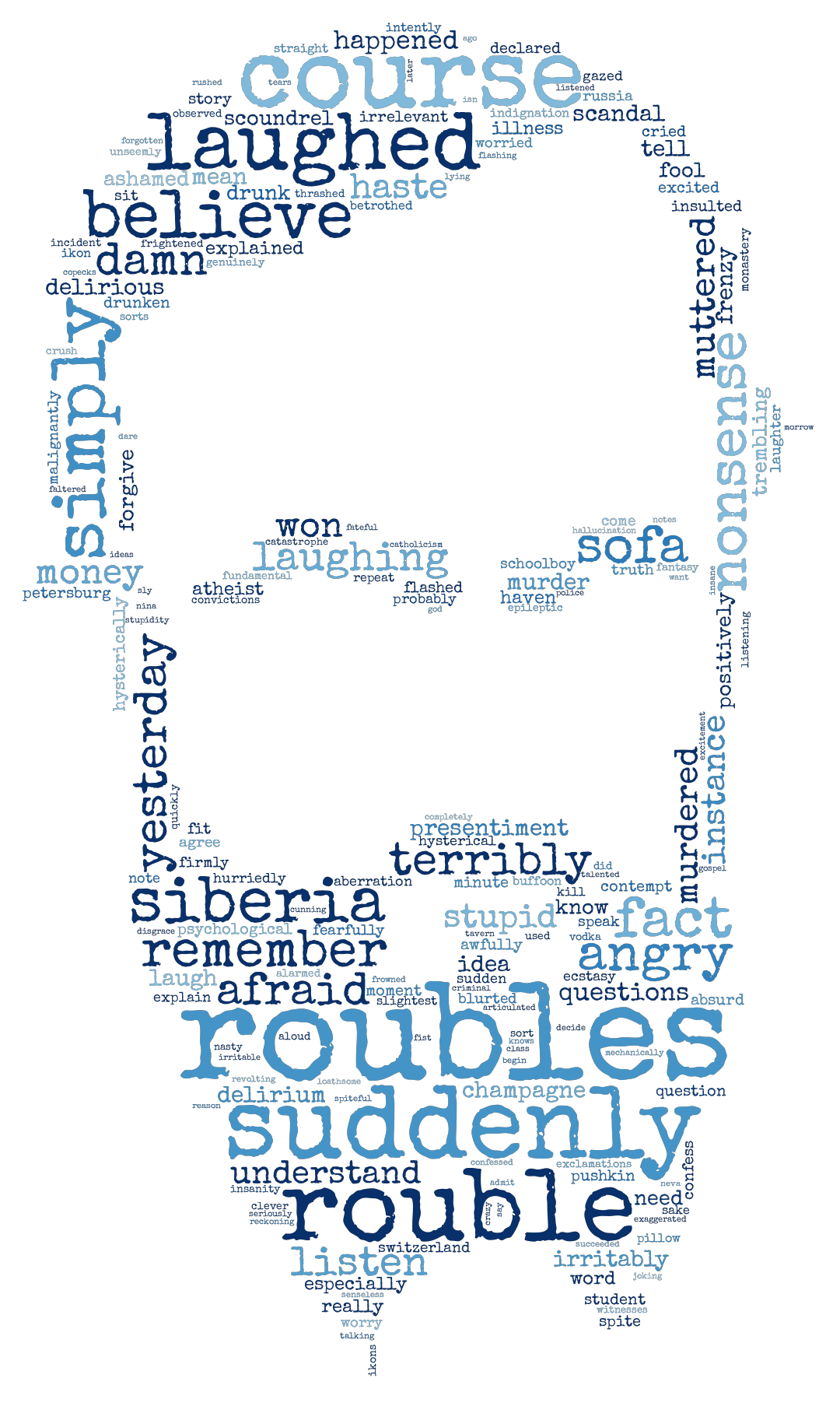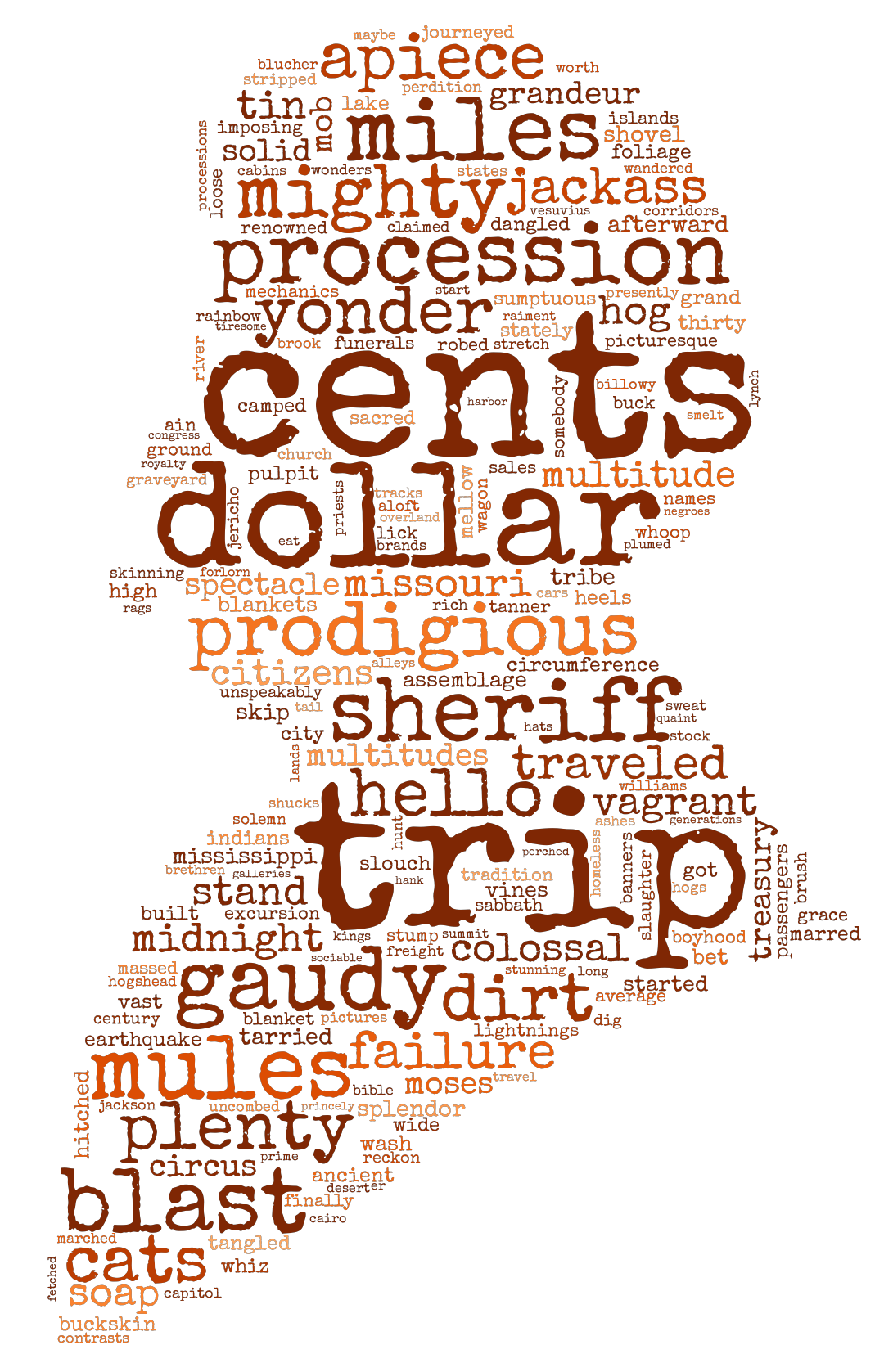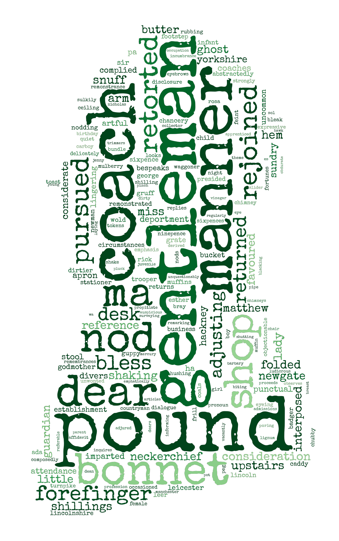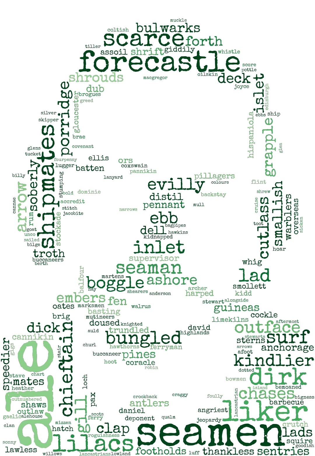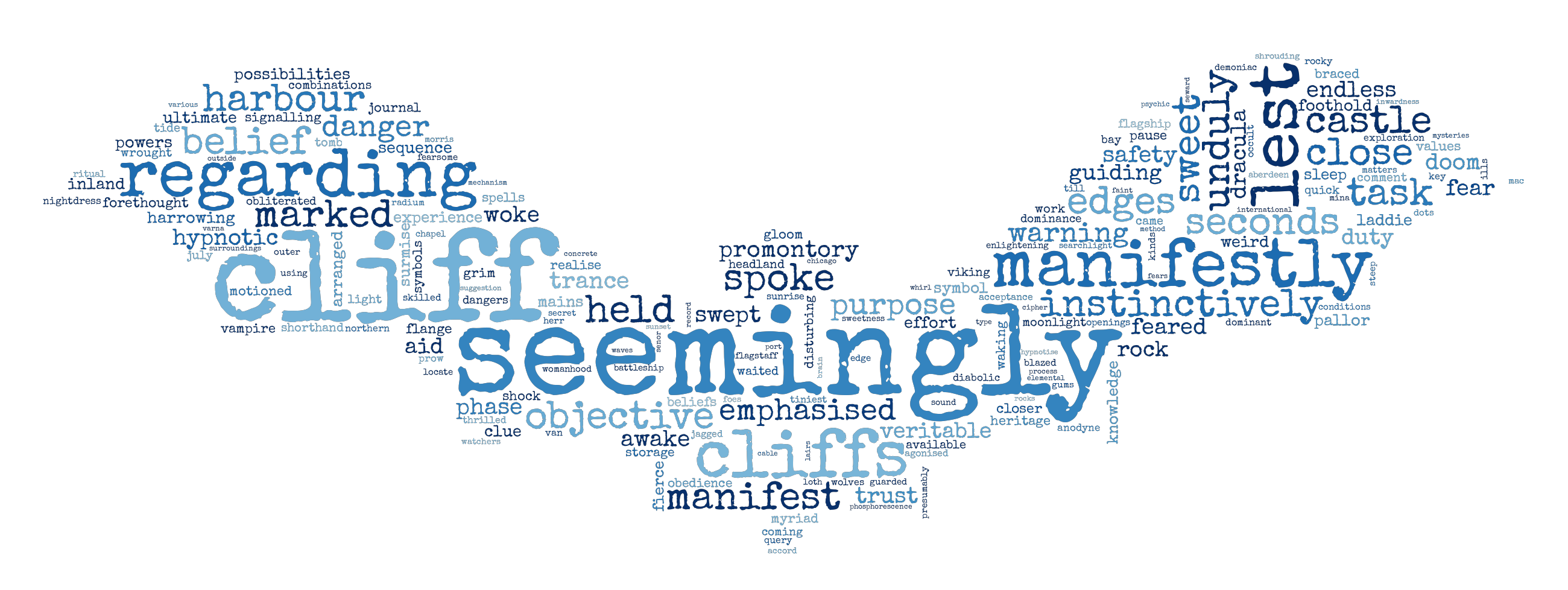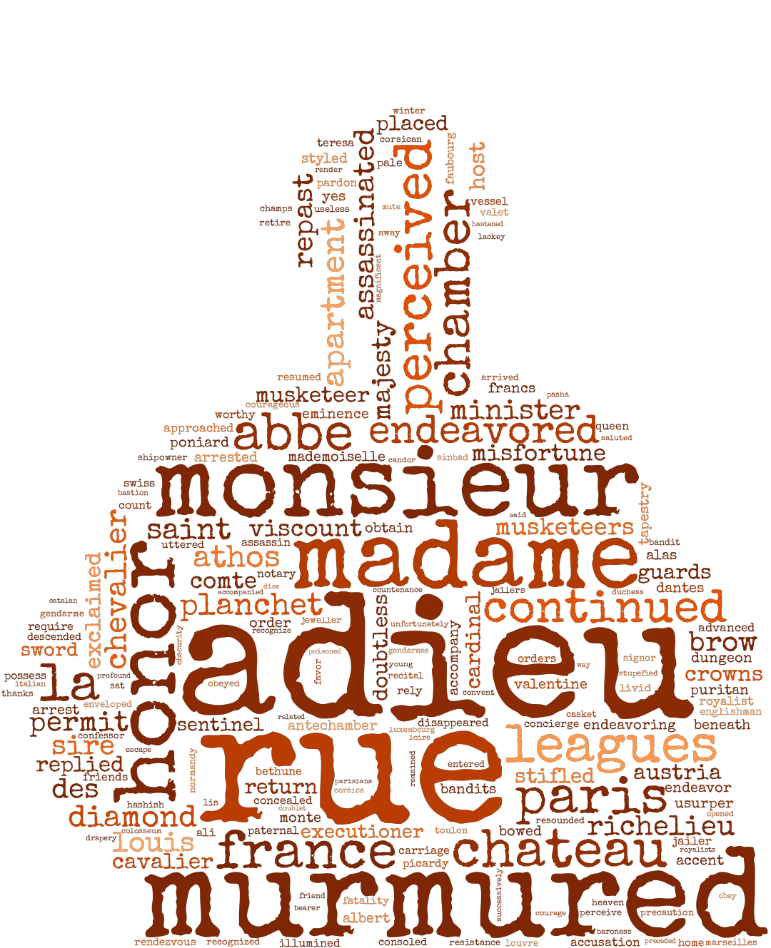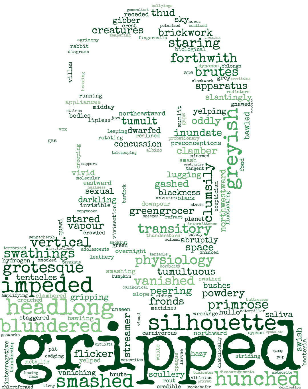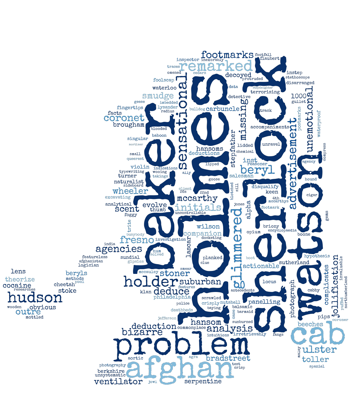
Figure 2: Generated Wordclouds

In order to prevent the wordclouds from being dominated by character names, a wide variety of books and authors should be used. The wordcloud for Doyle shows an example of this. Since Doyle writes almost exclusively about Sherlock Holmes, the classifier identifies words like Sherlock, Holmes, Watson as strong features. Authors that have different character names in their books do not suffer (or benefit) from this.

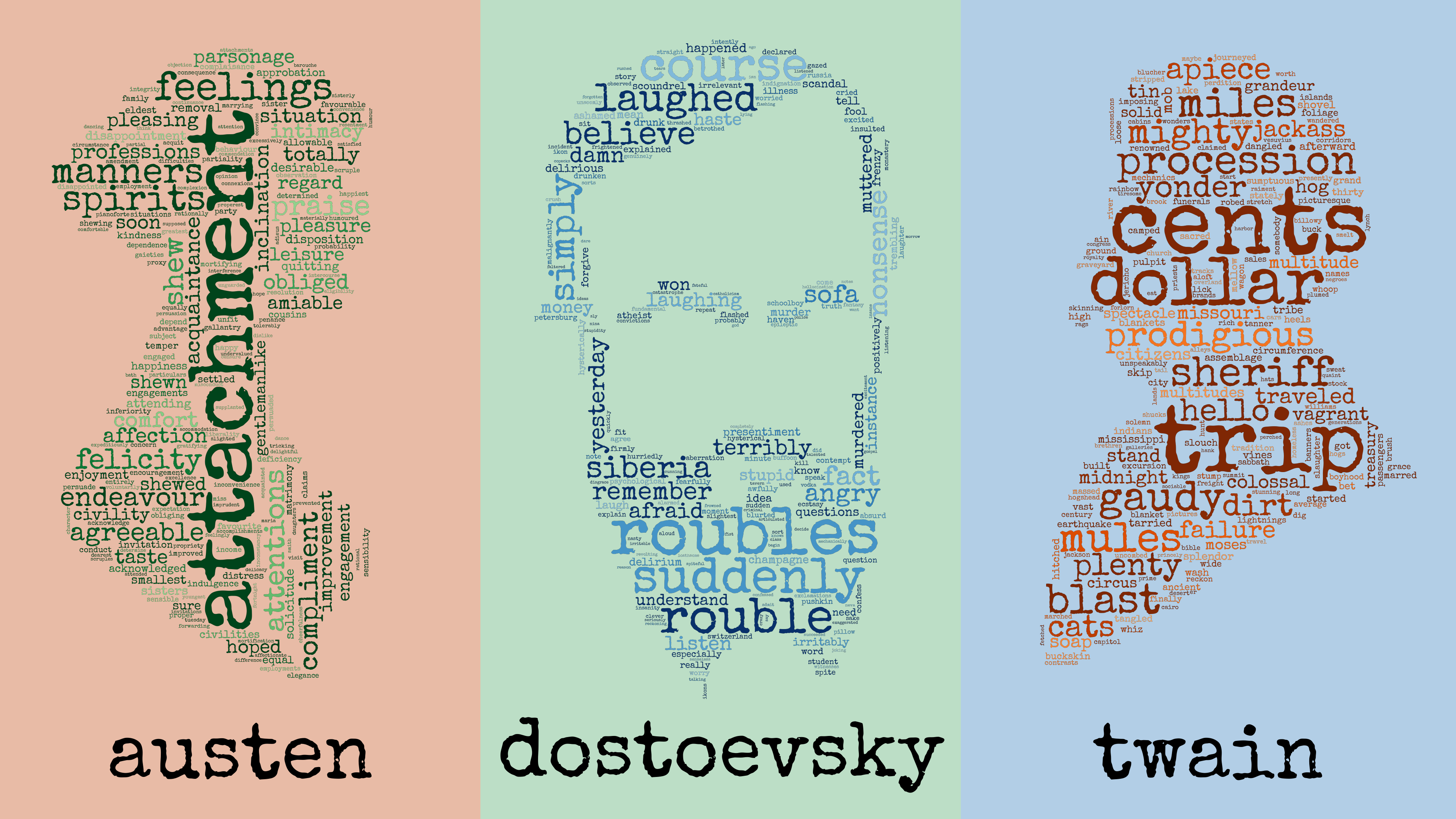
Figure 3: Full Version of Featured Image

A takeaway from the above is that gathering works from a wide variety of authors can improve results by making these types of uninteresting relationships more rare. For example, if only one author has a character named Tom, then the classifier may identify Tom as a strong feature for the author. This is technically correct, but probably not very interesting if the goal is to gain a deeper understanding of an author's style. Introducing more authors and books makes it more likely that multiple authors have a character named Tom, thus decreasing the importance of Tom as a feature for any one author.