Eigenfaces versus Fisherfaces on the Faces94 Database with Scikit-Learn

Thu, 18 Feb 2016

Biometrics, Computer Science, Facial Recognition, Machine Learning, Mathematics

In this post, two basic facial recognition techniques will be compared on the Faces94 database. Images from the Faces94 database are 180 by 200 pixels in resolution and were taken as the subjects were speaking to induce variations in the images. In order to train a classifier with the images, the raw pixel information is extracted, converted to grayscale, and flattened into vectors of dimension \(180 \times 200 = 36000\). For this experiment, 12 subjects will be used from the database with 20 files will be used per subject. Each subject is confined to a unique directory that contains only 20 image files.

import numpy as np
import matplotlib.pyplot as plt
from sklearn import cross_validation
from sklearn.discriminant_analysis import LinearDiscriminantAnalysis
from sklearn.decomposition import PCA
from random import randint
import matplotlib.cm as cm
from skimage import io, color
import os
# %% Read image data
numImg = 20
numSbj = 12
A = np.zeros([numImg * numSbj, 180 * 200])
y = np.zeros([numImg * numSbj])
fPath = #Path to face94 database
j = numSbj
c = 0
for i in os.listdir(fPath):
    if(j <= 0):
        break
    j -= 1
    for f in os.listdir(fPath + '/' + i):
        imgPath = fPath + '/' + i + '/' + f
        A[c, :] = color.rgb2gray(io.imread(imgPath)).reshape([1, 180 * 200])
        y[c] = j
        c = c + 1

Currently, each row in the matrix \(\textbf{A}\) corresponds to a single flattened image. The vector \(\textbf{y}\) indicates the corresponding subject ID (0 - 11).

Eigenfaces Based Classification

To compute the eigenfaces of these images, principal component analysis (PCA) is performed on the matrix \(\textbf{A}\). The eigenfaces are then the first \(n\) principal components of the matrix \(\textbf{A}\). This can be done in python as follows:

plt.figure()
pca = PCA(n_components=4)
pca.fit(A)
for i in range(4):
    ax = plt.subplot(2, 2, i + 1)
    ax.imshow(pca.components_[i].reshape([200, 180]))
plt.show()

The plot of the first four eigenfaces of the input data is as follows:

eigenfaces

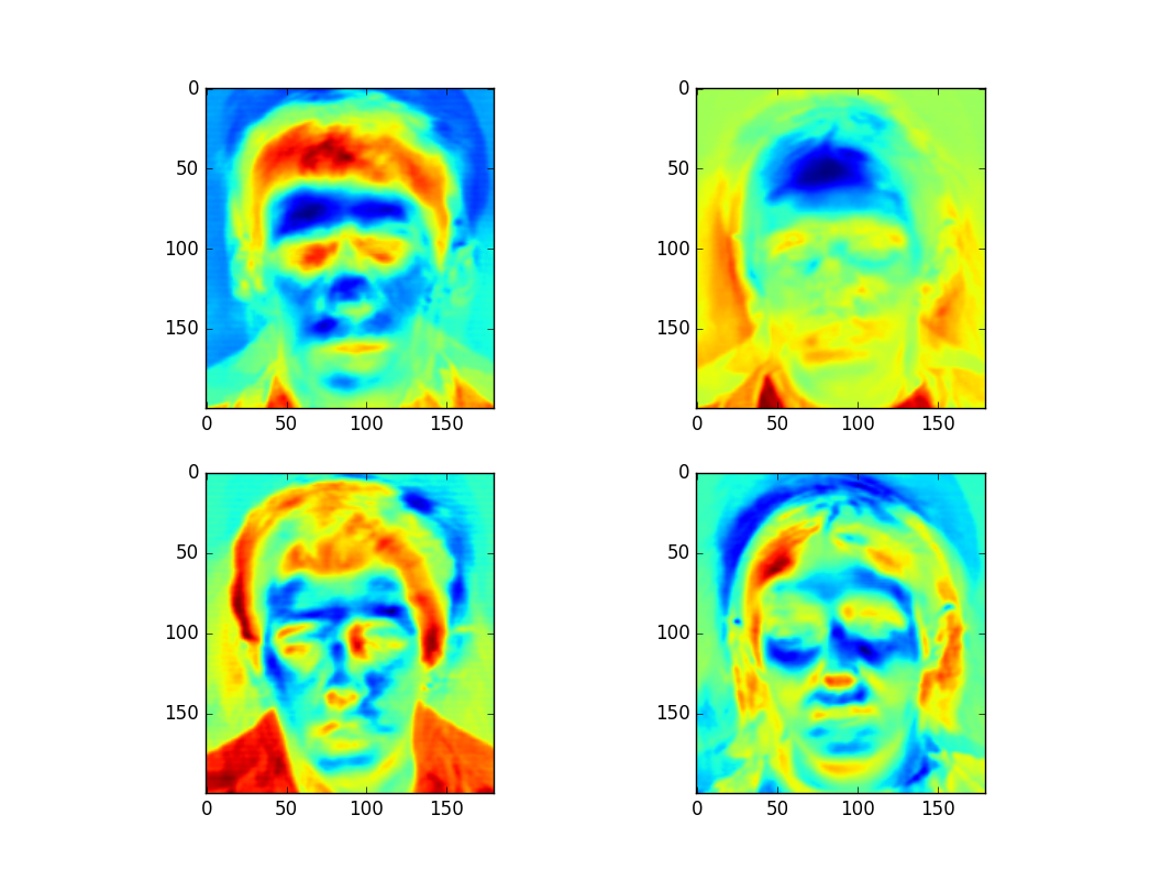
Figure 1: Plot of First Four Eigenfaces

Next, the data is approximated as a linear combination of the eigenfaces (principal components); only the weights of the eigenfaces are used to represent the data. Using more eigenfaces results in a better approximation. The following plot shows successively better approximations of an image using 1, 2, 3, and 4 eigenfaces (from top to bottom left to right).

eignLC

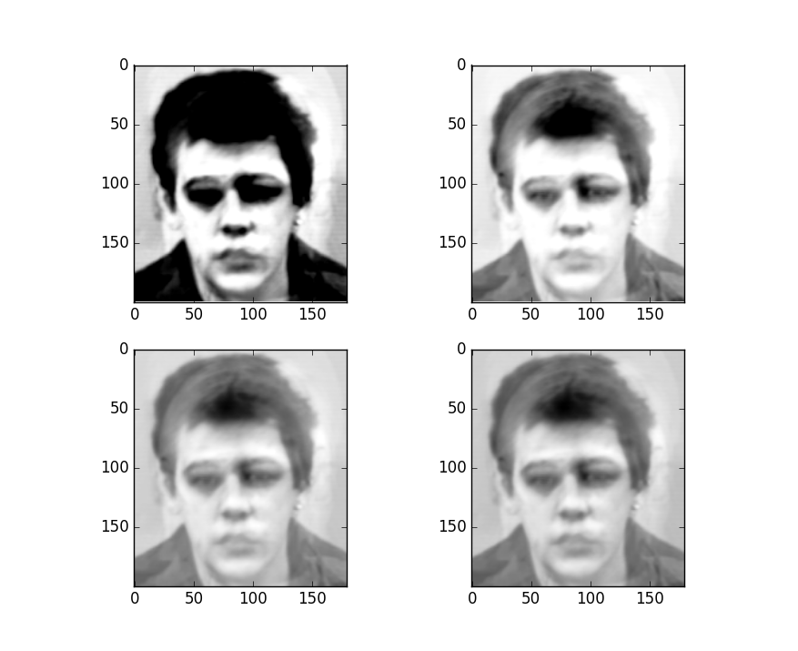
Figure 2: Successive Approximation of Input Image

By preserving a small number of eigenfaces, the dimension of the data can be greatly reduced. Classification can then be performed in this lower-dimensional space. For example, a K Nearest Neighbors classifier could be used. The transformed image data can be computed and plotted as follows (2 eigenfaces are preserved for a 2D plot):

#Colors for distinct individuals
cols = ['#{:06x}'.format(randint(0, 0xffffff)) for i in range(numSbj)]
pltCol = [cols[int(k)] for k in y]
# %% Plot 2d PCA data
drA = pca.transform(A)
plt.figure()
plt.scatter(drA[:, 0], drA[:, 1], color=pltCol)
plt.show()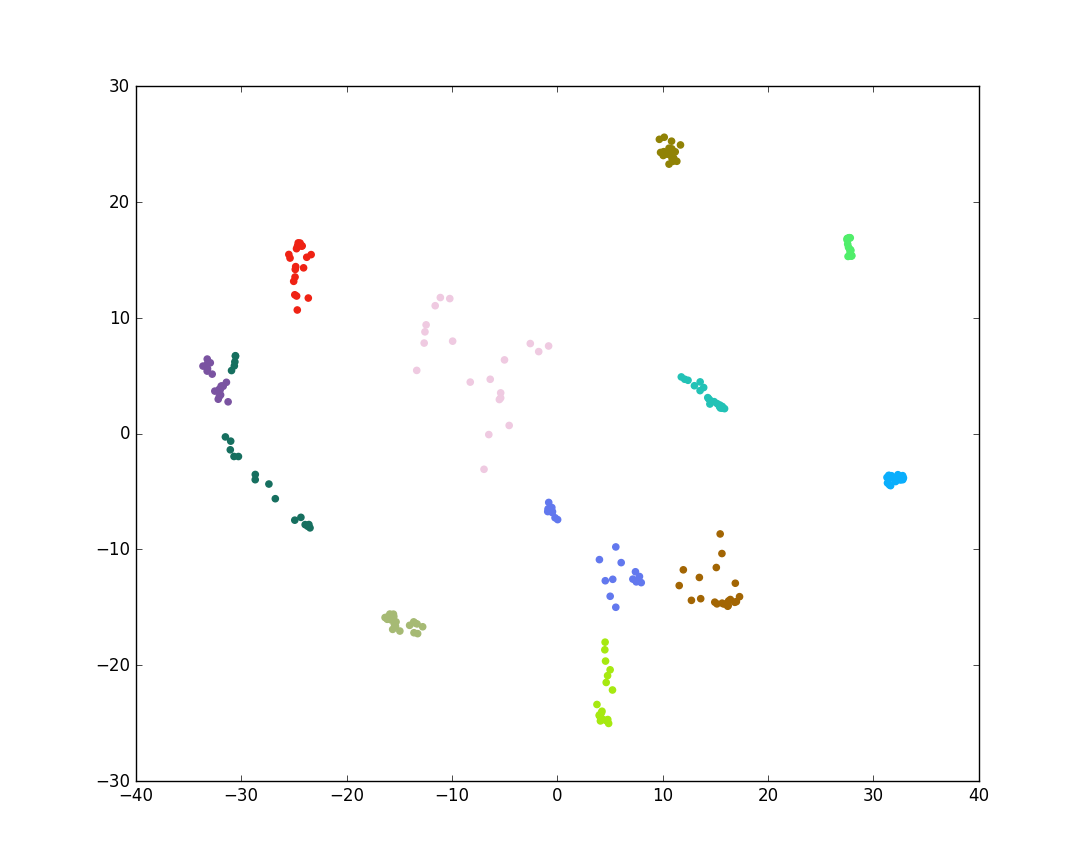

eignTrnsf

Figure 3: Plot of PCA Transformed Image Data

Notice in Figure 3 that the green and purple classes in the middle left overlap, however. This is not ideal. PCA finds a projection which maximizes the variability of all the data, but this does not take into account any class information. Linear discriminant analysis (LDA), on the other hand, maximizes the variability between each of the classes while also taking into account the variability within the classes themselves. For classification purposes, this is a better transformation. LDA based facial recognition is known as Fisherfaces.

Fisherfaces Based Classification

Fisherfaces are similar to eigenfaces, but LDA is performed on the input data matrix. From the last post, the LDA transform can be found by maximizing the Rayleigh quotient:

\[\displaylines{\max\limits_{a}\frac{a^{T}\textbf{B}a}{a^{T}\textbf{W}a}}\ ,\]

where

\[\displaylines{\textbf{W}=\sum\limits_{i=1}^{m}{\sum\limits_{j \in c_{i}}{(\textbf{x}_{j}-\boldsymbol{\mu}_{c_i})(\textbf{x}_{j}-\boldsymbol{\mu}_{c_i})^{T}}}}\ ,\]

is the within-class scatter matrix,

\[\displaylines{\textbf{B}=\sum\limits_{i=1}^{m}{N_{i}(\boldsymbol{\mu}_{c_i}-\overline{\textbf{x}})(\boldsymbol{\mu}_{c_i}-\overline{\textbf{x}})^{T}}}\ ,\]

is the between-class scatter matrix, \(N_{i}\) is the number of samples belonging to class \(c_{i}\), \(m\) is the number of classes, and \(\overline{\textbf{x}}\) is the mean vector of all input vectors.

However, with facial recognition the matrix \(\textbf{W}\) is (most likely) singular (and thus not invertible) since the number of samples \(m\) is typically much less than the number of features \(F\). With this experiment, there are \(F = 36,000\) pixels per image and only \(N = 240\) total samples (images). The Fisherfaces technique circumvents this problem by first applying PCA to transform the number of features from \(F\) to \(N-m\) before applying LDA on the transformed data. This can be accomplished in python as follows:

# %%Compute Fisherfaces
lda = LinearDiscriminantAnalysis()
#Use cross validation to check performance
k_fold = cross_validation.KFold(len(A), 3, shuffle=True)
for (trn, tst) in k_fold:
    #Use PCA to transform from dimension F to dimension N-m
    pca = PCA(n_components=(len(trn) - numSbj))
    pca.fit(A[trn])
    #Compute LDA of reduced data
    lda.fit(pca.transform(A[trn]), y[trn])
    yHat = lda.predict(pca.transform(A[tst]))
    #Compute classification error
    outVal = accuracy_score(y[tst], yHat)
    print('Score: ' + str(outVal))

Results from this code are given in the Results section. A plot of the Fisherfaces can be done as follows:

# %% Fit all data for plots
pca = PCA(n_components=(len(A) - numSbj))
pca.fit(A)
pcatA = pca.transform(A)
lda.fit(pcatA, y)
ldatA = lda.transform(pcatA)
#Plot fisherfaces
plt.figure()
for i in range(4):
    ax = plt.subplot(2, 2, i + 1)
    #Map from PCA space back to the original space (of images)
    C1 = pca.inverse_transform(lda.scalings_[:, i])
    C1.shape = [200, 180]
    ax.imshow(C1)
plt.show()

The Fisherfaces for this example are as follows:

fisherFace

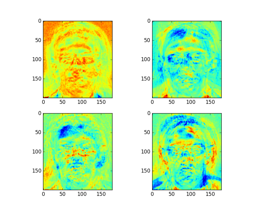
Figure 4: First Four Fisherfaces of Dataset

Results and Conclusion

The classification accuracies from each of the 3 tests are as follows:

Score: 1.0
Score: 0.9875
Score: 1.0

As can be seen, the classification accuracy is very high. This can be attributed to the well behaved nature of the classes in this instance. There is little variation in lighting and facial orientation which can both hurt performance. It should be noted that the initial PCA transform for Fisherfaces is not strictly necessary when using scikit-learn. Because scikit-learn does not directly invert the matrix \(\textbf{W}\), but instead uses a more sophisticated procedure, LDA can be directly performed on the input matrix, simplifying the code. The simplified code is as follows and plot of the transformed data are as follows:

# %% simplified LDA
k_fold = cross_validation.KFold(len(A), 3, shuffle=True)
for (trn, tst) in k_fold:
    #Compute LDA of reduced data
    lda.fit(A[trn], y[trn])
    #Compute classification error
    outVal = lda.score(A[tst], y[tst])
    print('Score: ' + str(outVal))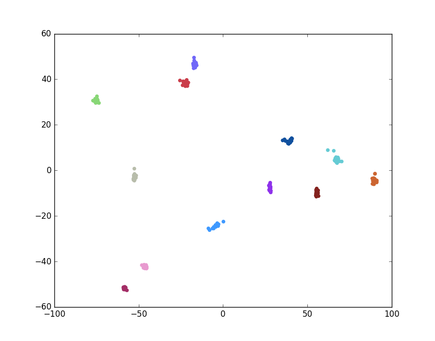

ldaPlt

Figure 5: Plot of LDA Transformed Images

In the above plot, different colors denote different classes (individuals). Indeed, the above method is preferable as it typically allows for perfect performance (100% accuracy) on this dataset.

References

Belhumeur, Peter N., João P. Hespanha, and David J. Kriegman. "Eigenfaces vs. fisherfaces: Recognition using class specific linear projection." Pattern Analysis and Machine Intelligence, IEEE Transactions on 19.7 (1997): 711-720.